CREW repository

Welcome to the CREW repository. The CREW repository contains several types of data, which are useful to be shared with other experimenters. Following types of data are available in the CREW repository:

full experiment descriptions: when reading reports containing experimental results, it is often difficult or impossible to verify the claims of the author or to use the experiment as a base for further research. Full experiment descriptions contain all information needed to run a particular experiment. By publishing full experiment descriptions, we aim for more transparent and thus more valuable experimentation results. Furthermore, the possibility to re-use experiment descriptions enables fair comparison (benchmarking) of wireless solutions.
traces: traces are files describing wireless traffic of heterogeneous technologies, either at packet level (e.g. a timed sequence of Bluetooth packets, a certain profile of Wi-Fi use, the activity of a primary LTE user), or data recorded at spectrum level (e.g. recorded spectrum use in a certain location over time, artificially created patterns containing reference interference on a particular frequency).
background environments: background environments are configurations that can be used to create repeatable wireless environments and are tied to a particular testbed. The configuration files of these background environments link particular traces (see above) to particular nodes at particular times, inside a particular testbed.
processing scripts: useful scripts (in multiple scripting languages, matlab, java,...) that, for example, convert the output of a certain type of commercially available tool or CREW component to the CREW common data format.
performance metrics and benchmarking scores: detailed descriptions of performance metrics and measurement methodologies. Benchmarking scores are abstractions derived by combining different performance metrics. These scores may be useful to when comparing a large set of solutions or for automated decision making during an automated benchmarking process.

The CREW repository is currently being populated by members of the CREW consortium. In this early stage of development, it is currently not possible for external experimenters to directly contribute to the repository. If you want to contribute your data to the repository, please contact us. In a later phase, it will either be possible to directly contribute to the CREW repository, or, CREW may decide to migrate its data with existing open repositories such as CRAWDAD.

Usage policy

The data available on the CREW repository may be used for your research, educational and commercial purposes. Unless specified otherwise, copying and modifying the data is allowed, as long as a reference to the CREW project or CREW repository (www.crew-project.eu/repository) is included. In addition, any other references to the original authors that might be included in the data should not be removed. When data from the repository is used in publications, CREW should also be referenced.

traces

Measurement traces that were captured during experiments are availabe for further evaluation. The data can be downloaded directly or if no link is availabe please contact the CREW responisble for further directions on how to obtain the trace files.

LTE Testbed Reference Data

Primary user test signals

These LTE testbed traces are provided in Matlab format and contain a structure with all relevant system parameters as well as a vector of I-Q samples. They can be used to check compatability with the LTE equipment at TUD.

TVWS experiment Logatec

The measurement traces for the Logatec experiment are available upon request. The results are stored in the CREW common data format.

In the TVWS the results are available for:

VESNA
USRP
IMEC sensing engine

Additionally ISM band activity was monitored using the TelosB nodes, also available in CREW common data format. Furthermore a GPS trace of the route that was followed is available, including signal strength predictions using a Longley-Rice channel model and hataDEM model implemented in the Grass-RaPlaT (http://www-e6.ijs.si/en/software/grass-raplat) propagation tool.

background environments

Background environments for use at w-iLab.t Zwijnaarde

Name	Description	File(s)
wilab-home-1	The home Environment is emulated using 4 WiFi embedded PCs. A server, email client, data client, and video client. The server acts as a WiFi access point and a gateway for the emulated services. The email client will “check email” once every 15 seconds for a duration of one second. The data client is emulated via TCP streams one starting at 45 seconds for a duration of 22.5 seconds and the other starting at 105 seconds for a duration of 45 seconds. The video client is emulated as a UDP stream of 100 kbps for half the experiment cycle and it will start at the middle of the experiment. In total, the experiment takes 150 seconds.	iperfED_ENV.rb iperfED_ENV.json
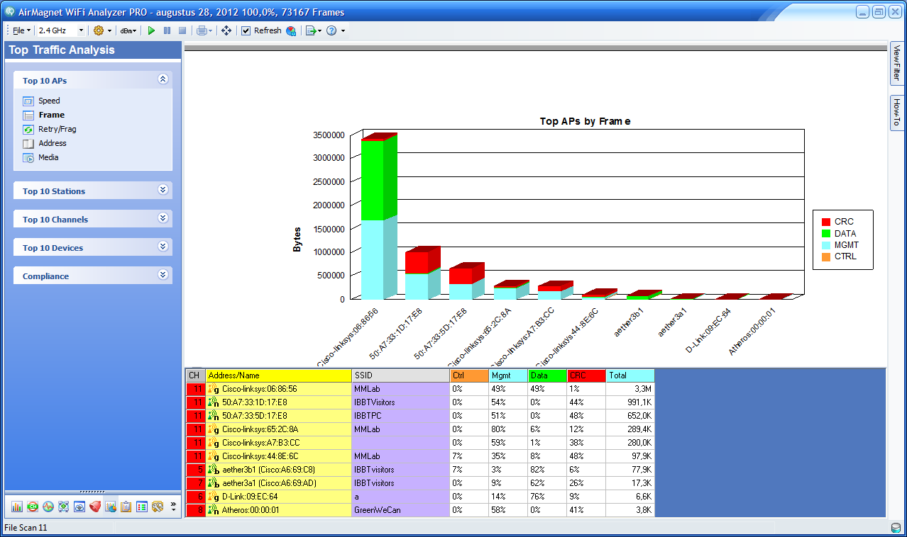
wilab-office-1	The office environement is based on a live capture performed with Airmagnet. Due to the limitation of complexity and involved number of nodes, we only selected the most active access points to emulate. In the wilab office 1 environment, three access points were emulated: ibbtvisitor (ather3a, associated with 7 clients), ibbtvisitor (ather3b, associated with 7 clients), and MMlab (associated with 6 clients). 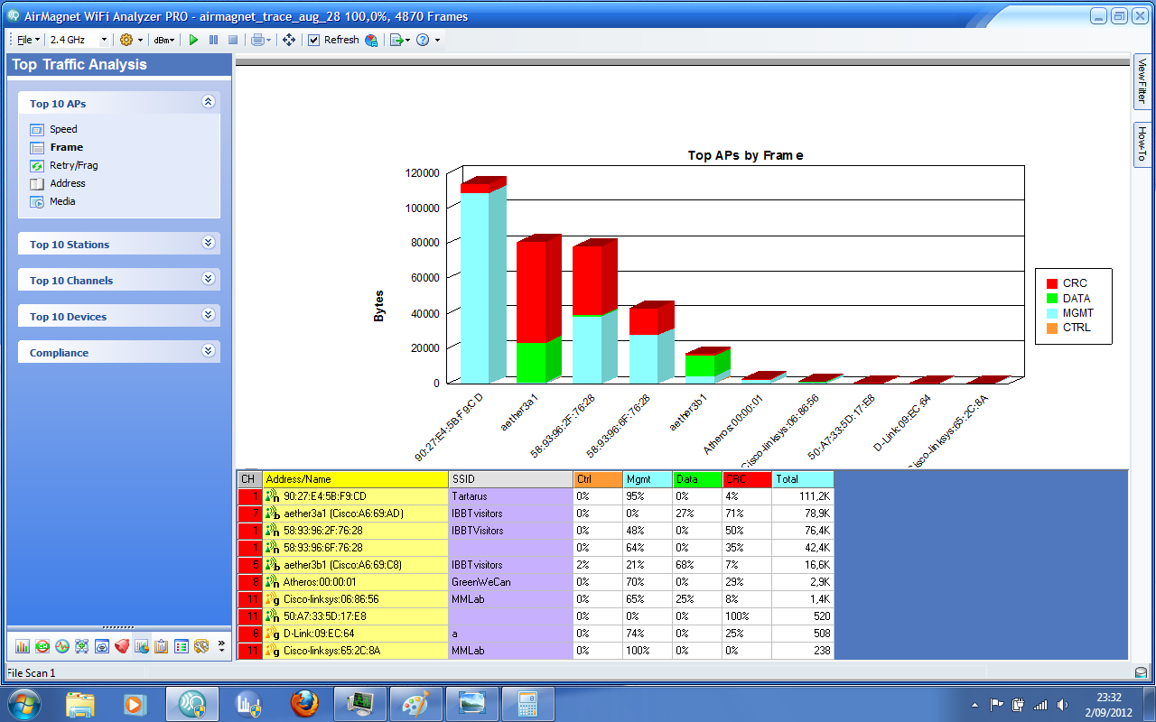The airmagnet trace file and its corresponding omf script are attached	office_1.rb office1_ap.png office1.amm
wilab-office-2	Simlar to wilab office 1 environment, office 2 environment is again based on another live capture of Airmagnet device, this time only the ibbtvisitor network (2 access points and 8 clients) is emulated. More information can be seen in the Airmagnet trace	office_2.rb office2_ap.png office2.amm
wilab-office-3	An office environment created based on office 1 and office 2 scenario, consists of 4 Access Points and several Bluetooth devices	office_3.rb office_3.xml
ISR-Tutorial	XML experiment configuration file used in CREW experiment definition tool tutorial.	ISR.xml

experiment descriptions

Experiment descriptions are obviously very specific.

To view the XML schema for experiment description, please refer to http://www.crew-project.eu/cdf_xml/schema.html

For some examples, please browse through one of the experiments below:

Multi-antenna LTE sensing

Sensitivity measurement

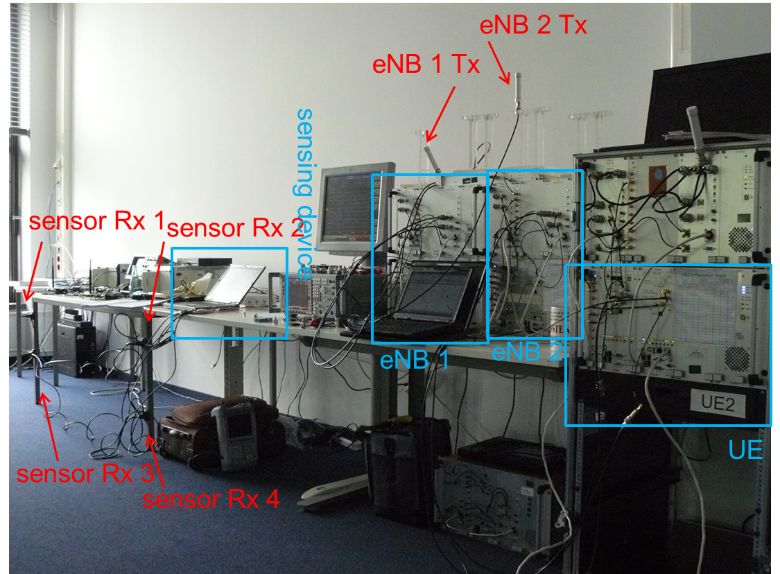
This experiment derives from a metrology use case, where the multi-antenna sensing device can be used for downlink interference analysis of LTE cellular networks. The process consists of creating a list of the received signals on an LTE channel as well as obtaining their physical characteristics and identifying the base stations which are transmitting these signals. Interference analysis is based on the smart antennas approach employing an array of antennas. When this antenna array receives several sources emitted by different base stations, the signals are recombined in order to detect and demodulate each received source, while the other received signals are considered as interference that can be rejected when it comes from different directions. Since the matched filter approach is used for detection, the signal can be demodulated and system parameters like the physical layer cell identity, cyclic prefix length, duplex mode, base station signal level, Ec/I0, as well as time and frequency channel impulse response can be determined. The goal of the experiment is is to demonstrate the detection algorithm and hardware, as well as show the multi-antenna processing gain over a mono antenna sensing scenario.

Interference rejection measurement

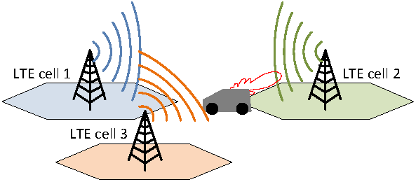
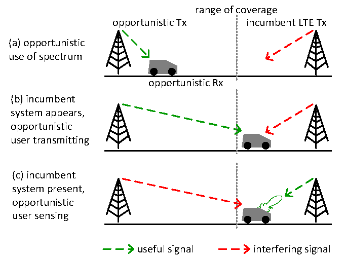
LTE detection with spatial interference rejection capabilities can also be useful for sensing in CR environments. Consider a mobile opportunistic receiver (Rx) uses a white space in a certain frequency band that is available at a particular geographic location (a). The system has to check periodically for the presence of an incumbent user that might be utilizing that band. When the mobile opportunistic Rx moves to a location where the white space is no longer available, it receives the signal from the incumbent LTE transmitter (Tx). While the opportunistic system is not aware of the presence of the incumbent Tx, it is still communicating and for the opportunistic Rx, the signal coming from the incumbent Tx is considered as interference (b). When the opportunistic Rx senses the spectrum, the signal coming from the incumbent LTE Tx is now the signal of interest and the signal from the opportunistic Tx the interference, as it is jamming the sensing process (c). Typically, during this process silent periods are allocated in the opportunistic system waveform, in order to perform sensing without being jammed by its own system. But sensing can also be performed simultaneously with the data transfer, if the opportunistic Rx has interference rejection capabilities, i.e. by using an antenna-array and antenna processing algorithms. The goal of this experiment is to demonstrate the interference rejection capabilities of the multi-antenna sensing platform

Setup Overview

Files

Experiment description in common data format: JSON | XML

VESNA spectrum sensing in ISM 2.4GHz

VESNA spectrum sensing in ISM 2.4GHz in the Log-a-tec testbed

The Log-a-tec testbed supports experiments in ISM 868 MHz and 2.4 GHz and in UHF bands. In the ISM remote sensing and transmissions are possible while in the UHF only remote sensing is possible. For transmission on UHF bands, remotely emulating a wireless microphones with ISM 868 transmitters is possible while for anything more advanced, transmitters needs to be taken in the field (JSI has license to transmit in UHF bands).

In the following, we discuss an ISM 2.4 GHz experiment description performed in the Log-a-tec industrial zone cluster depicted in the figure below.

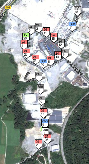
The experiment scenario is as follows. Three VESNA nodes (ids 25, 6, 4) from the Log-a-tec testbed are configured to perform spectrum sensing in the 2.4 GHz spectrum band. Four VESNA nodes (ids 2, 17, 24, 26) from the same testbed are configured to perform transmissions, each on a 200KHz channel in the 2.4 GHz band. The transmissions are performed in channels 50, 105, 155 and 205 and they start 5 seconds after the sensors start sensing the environment and end 5 seconds before the sensors stop sensing.

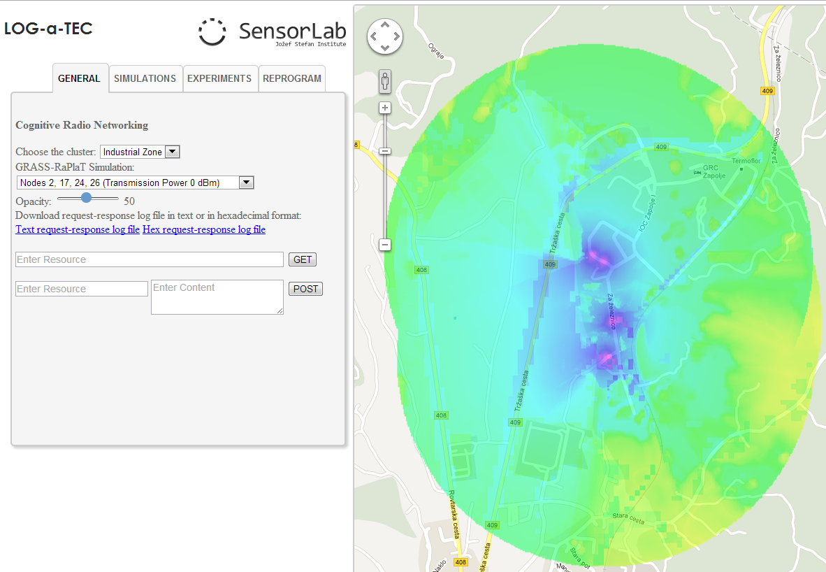
The portal facilitating the experiment configuration is presented in the figure below while the experiment description in CREW common data format are available in XML and JSON encoding below.

Files

Experiment description in common data format: JSON | XML

Attachment	Size
VESNA_SS_24GHz.json	13.29 KB
VESNA_SS_24GHz.zip	2.34 KB
IndustrialZoneCluster.png	308.52 KB
VESNA_SS_24GHz.png	284.29 KB

Wi-Fi throughput experiments

WI-FI throughput experiment

In the following experiment we examine WI-FI throughput performance under various interference conditions. In all experiments the throughput is logged as performance metric.

Name	Description	Files
Distributed Sensing for identify hidden terminal effect	This experiment involves two pairs of WI-FI nodes, located far away. We monitor the environment both with packet sniffing and distributed sensing via USRP sensing engine. One WI-FI group is considered system under test (SUT) while the other is considered as Interferer (INT). The transmit power of INT group is varied from 0 dBm to 20 dBm in step of 2 dBm, controlled via the benchmarking framework. It is seen that there is a interval where packet sniffing do not detect INT activity but distributed sensing can.	xmlfiles.tar iriswrap.tar hiddenterminalEd.rb tcpdumpwrap.tar
Interference caused by overlapping WI-FI channel	This experiment involves two pairs of WI-FI nodes, they operate on adjacent WI-FI channels. The amount of overlapping between the two pairs are controlled via benchmarking framework. The rarget is to find out how does WI-FI react to interference caused by WI-FI activities on the adjacent WI-FI channel	xmlfiles.tar tcpdumpwrap.tar tcpdumpwrap.tar channelOverlapping.rb
Interference caused by zigbee device	This experiment involves only one pair WI-FI nodes. An narrow-band interference signal is generated by a nearby zigbee node	jammer_mil2.tar iperfweiED_zb.rb tcpdumpwrap.tar

scripts

Scripts to produce CREW common data format (CDF) for spectrum sensing are available for different devices (Airmagnet, USRP SE, imec SE, Vesna, Telos, Wispy etc.). Other processing scripts to calculate power, create plot data etc are available too.

They can be found on github.

Performance metrics and scores

If nothing is measured during an experiment, the experiment makes little sense. Experimenters characterize the performance of their solution under test by recording a set of performance metrics. This overview presents a selection of metrics that may be of use for experimenters during the execution of their experiments.

This section provides both descriptions of performance metrics and of scores, which are higher level abstractions of one or multiple performance metrics. There are two main reasons why sharing these metrics is relevant:

it helps experimenters to build their experiments using unambiguously defined metrics (less effort, better definition).
it improves the comparability of results between experiments carried out by different experimenters (or at different times).

The metrics and below are organized in different categories.

1. Metrics

1.1 Spectrum characterization and Spectrum sensing

Name	Unit	Explanation / relevance	Formula or methodology	Comments
Channel duty cycle	ms	The channel duty cycle is defined as the ratio of time a channel is "occupied" over a given interval. A channel is considered "occupied" when the measured energy is above a certain threshold value Eth.	T(E>Eth)/Ti, where E is the measured energy over a certain channel for the specified interval, Eth is the energy threshold threshold, T(E>Eth) denotes the time when measured energy is above the treshold and Ti is the selected time interval
Received Signal Strength Indicator (RSSI) for VESNA	dBm	The RSSI indicates the power of the received signal as measured by the device. If only noise is present on the communication channel, this value equals the noise floor. This metric is relevant from two points of view: 1) it helps monitoring the sensitivity of the receiver over time 2) characterize the transmission channel for known transmitters.	The value is retrieved from the receiver (the CC chips).	RSSI data from sensing devices can be processed to obtain a periodogram (received power level vs. frequency and time). This holds for energy based detection methods and applies to VESNA sensor nodes. In order to characterize the radio environment, these will be compared to the transmitting part that is under the control of the testbed.
Probability of false transmission detection (PFTD)	%	The probability of false transmission detection represents the ratio between the number of false transmission detection reports vs the total number of transmission detection reports. It reflects the probability that the device reports that a transmission is present on the monitored channel without this transmission actually being present. In other words, the probability of the device erroneously reporting a transmission.	This value is computed as the ratio between false detection reports vs the total number of detection reports over a predefined time interval.	PFTD is dependent on the RSSI values as these are the values based on which the device decides whether a transmission is present ot not. This holds for energy based detection methods and applies to VESNA sensor nodes.
Probability of correct transmission detection (PCTD)	%	The probability of correct transmission detection represents the ratio between number of correct detection reports vs the total number of detection reports.	1-PFTD
Probability of missed transmission detection (PMTD)	%	The probability of missed transmission detection represents the ratio between false silence reports vs the total number of silence reports. It reflects the probability that the device reports that a transmission is not present on the monitored channel while a transmission is actually taking place on the channel. In other words, the probability of the device erroneously reporting a free channel.	This value is computed as the ratio between false silence reports vs the total number of silence reports over a predefined time interval.	PMTD is dependent on the RSSI values as these are the values based on which the device decides whether a transmission is present ot not. This holds for energy based detection methods and applies, among other things, to VESNA sensor nodes.
Probability of correct silence detection (PCSD)	%	The probability of correct silence detection represents the ratio between number of correct silence reports vs the total number of silence reports.	1-PMTD
Time to detection (TD)	ms	The time required that the sensing device detects an existing transmission in a given band. This metric is useful, among others, in estimating how long a sensing device from the secondary user's equipment needs to detect the transmission coming from a primary user.	Assuming band B is of interest, this value is measured a follows. 1) The sensing device listens to the activity in band B. 2) A known transmitter starts transmitting on B at time T1. 3) The sensing device detects the transmission at time T2. 4) The value of TD is: TD = T2 - T1.	TD is also dependent of RSSI values. This holds for energy based detection methods and applies, among other things, to VESNA sensor nodes.
Time to clear the spectrum (TCS)	ms	The time required that a transmitted vacates a given band. This is particularly useful for the cases when the secondary user needs to move away from a band dedicated to the primary user.	Assuming band B is of interest, this value is measured a follows. 1) A sensing device listens to the activity in band B where a known transmitter T is transmitting. 2) The transmitter T receives a command instructing it to stop transmission on B at time T1. 3) The sensing device detects that transmitter T stopped transmitting in B at time T2. 4) The value of TCS is: TCS = T2 - TD - T1.	TCS is also dependent of RSSI values. This holds for energy based detection methods and applies, among other things, to VESNA sensor nodes.
Probability of correct hidden node localization (PCHNL)	%	The probability that the hidden node is correctly localized.	The value is computed as the ratio between the number of times the known location of a hidden node has been detected correctly versus the total number of detections.
Probability of incorrect hidden node localization (PICHNL)	%	The probability that the hidden node is incorrectly localized.	The value is computed as the ratio between the number of times the known location of a hidden node has been detected incorrectly versus the total number of detections.

1.2 Networking

Name	Unit	Explanation / relevance	Formula or methodology	Comments
Application layer packet delay	ms	measures the time needed for a packet to arrive at the application layer at a certain node B after being sent from the application layer at node A.	1/ record timestamp as packet leaves the application layer of node A. 2/ record (synchronized) timestamp when packet is received by node B. 3/ calculate the difference
Link packet reception rate (LPRR)		The Link packet reception rate over a single link is defined as the ratio of received packets at the end node of the link over the number of transmitted packets transmitted by the source node of the link. The End-to-end PRR is calculated as the product of the reception rates on each link along a path in the network	LPRR_i = num_of_packet_received_i /num_of_packets_transmited (i is the index of the link segments in a multihop routes), LPRR_e2e= PRR_1PRR_2…PRR_N (N is the total number of link)
Link packet error rate (LPER)		The packet error rate over a single link is defined as the ratio of lost packets over the total amount of transmitted packets over that link.	LPER = sum(lost packets) /num_tx_packets = 1- LPRR
Packet Jitter	ms	We define jitter as the variation of a packet delay with respect to the application layer packet delay. In CR can be high and therefore cause problems to the steraming applications.	Based on the application layer packet delay measurements it is possible to calulate average and variance of the metric.

1.3 Metrics specifically related to the imec Sensing Agent

Name	Unit	Explanation / relevance	Formula or methodology	Comments
FFT based RSSI (IMEC Sensing Engine)	dBm	RSSI value based on FFT on time domain signal which is retrieved from the Sensing Engine. The bandwidth to which the values apply depends on the number of points selected in the FFT and bandwidth of the RF front-end. Currently the SE API supports 20 MHz bandwidth and 128 point FFT which results in a corresponding bandwidth for each value of 156.25kHz	See (1)	1) Since the FFT uses the baseband time domain signal saturation effects in the RF sections may become invisible and corrupt the result 2) The dBm values have been calibrated for the maximum gain setting of the RF front-end
Baseband time domain power measurements (IMEC Sensing Engine)		Depending on the configuration (WLAN G, ZigBEE, WLAN A, BlueTooth, 2 or 4MHz in ISM band) a power measurement is executed for the desired channel bandwidth and RF frequency. The result is a unitless number which is the sum of the powers of 32 time-domain samples.	See (1)	Since value heavily depends on the used gain settings in the RF section, reference curves are available to convert the unitless values to dBm
Cyclostationary detection for DVB-T signal (IMEC Sensing Engine)		Outcome of cyclostationary detection on DVB-T signal. Two modes are supported, 2k and 8k carriers and multiple cyclic prefix lengths are supported (1/4, 1/8, 1/16 and /1/32)	See (1) and (2)

http://www.crew-project.eu/sites/default/files/SensingEngine_UserManual.pdf
“Performance evaluation of sensing solutions for LTE and DVB-T”, Van Wesemael, P.; Pollin, S.; Lopez Estraviz, E. and Dejonghe, A., IEEE Symposium on New Frontiers in Dynamic Spectrum Access Networks – DySPAN 2011

1.4 Other

Name	Unit	Explanation / relevance	Formula or methodology	Comments
Node energy consumption (P)	mW	The node energy consumption indicates how much energy is consumed by this node at a certain moment. In wireless sensor networks, there is a trade off between the desired network performance and energy consumption. Hence it is wise to deliberately put sensor in sleep mode and only wake up from time to time.	1/ Direct measurement: P=UI (measure the output voltage U and the current I provided by the battery or other power source) 2/ Indirect measurement: P=QP1+(1-Q)*P2 (Where Q is the sleeping duty cycle of the sensor node), P1 is the power consumption during sleep mode and P2 is the power consumption when it's in full operation	There are many additional ways to measure energy consumption, the provided formulas and methodology only shows the most common ones.
Memory consumption	byte	Program memory (flash) consumption as well as RAM size of a software component are especially important in the context of evaluating resource-constraint platforms, such as sensor networks. The numbers are given in byte and can either be for specific software components (e.g. representing a protocol) or for the entire image.	Typically the compiler will list the memory usage (Flash/RAM) of the overall application. Otherwise the binary may be inspected with tools such as objdump to retrieve memory consumption.
Physical Source Lines Of Code		Sometimes not only memory consumption but also the physical number of source lines of code (PSLOC) are an important metric to evaluate a solution. For example, PSLOC may give an indication how complex/difficult it may be to use a certain service from another client.	PSLOC are typically computed by a dedicated script that counts relevant line numbers for a specific programming language, more precisely "a physical source line of code is a line ending in a newline or end-of-file marker, and which contains at least one non-whitespace non-comment character.'' (http://www.dwheeler.com/sloc/redhat71-v1/redhat71sloc.html)	The following tool supports a large number of program languages: http://www.dwheeler.com/sloc (Wheeler, D.A.: Counting source lines of code (SLOC))

2. Scores

A score is an abstract representation of the experiment result. A score is a higher level abstraction of performance metrics. Within the CREW benchmarking concept, the score of an experiment is scaled between 0 to 10, with 10 representing the perfect performance for a certain characteristic, and 0 for the opposite performance.

Name

Description

Script

Score for large scale CTP sensor network performance

A large scale collection tree protocol (CTP) sensor network typically consists of multiple routes and each route has multi hops, it is difficult to say how the overall network is performing. Therefore we calculate end-to-end packet reception rate for each sensor node. For a node that is only one hop away from the sink node, the end-to-end PRR is the PRR on the final link. For a node located two hop from the sink, the end-to-end PRR refers to the product of the PRR on two links, etc. Finally the end-to-end PRR is averaged among all the none-sink nodes. The averaged PRR can maximum reach 1, therefore the scaling factor is 10. The MATLAB script is attached for clarification

prr_perlink.m

score.m

Pre/Post experiment threshold score

Pre and Post experiments are used to estimate environment interference and thus easily select outlier experiments. Inside CREW experiment execution tool when pre/post experimentation is selected, a threshold score will be calculated after the end of each experiment run. The tool generates 9 threshold scores starting from -55dbm to -95dbm with a step of 5dbm level. A very high score (closer to 10), on any threshold level indicates that the environment is not interfered by a signal with strength above the given threshold dbm value.