CREW benchmarking tools
This section explains the use of CREW benchmarking tools
The CREW benchmarking tools allow experimenters an easy setup, execution, and analysis of experiments that will be carried out on CREW federated testbeds. Currently, the tools are implemented in iMinds testbed and in short time it will be available to the other CREW testbeds. The tools are generic and easily portable to other testbeds with minor effort.
In order to be able to access to the CREW benchmarking tools running at the iMinds w-iLab.t Zwijnaarde testbed, a VPN account is needed. For information on how to obtain an account to w-iLab.t, please consult the following page.
CREW benchmarking tool list:
Easy experiment configuration
Tool Location (OpenVPN required) http://ec.wilab2.ilabt.iminds.be/CREW_BM/BM_tools/exprDef.html
The experiment definition tool allows the experimenter to configure the system under test and the wireless background environment. Two types of configuration are possible. One can start from scratch and create a full experiment definition or configure from an existing one.
For the latter case, a number of solution under test and background environment configuration files are stored in CREW repository.
For detail explanation, refer the section CREW experiment definition.
Experiment Definition Tool
The experiment definition tool is used to define, configure, and make changes to wireless experiments that are to be conducted on different testbeds. Before explaining the experiment definition in detail, an experimenter need to be familiar with the concept of experiment resource grouping. This concept is taken from the cOntrol and Management Framework (OMF) developed by the collaborative effort of NICTA and Winlab [1].
The experiment resource grouping concept treats an experiment as a collection of resources aggregated into groups. Resources can be any of these but not limited to WI-FI nodes, sensor nodes, spectrum sensing devices, and software-defined radios. With in a group, multiple nodes run different applications that were predefined in an application pool. And a single application as well defines a number of optional measurement points. In figure 1, we show a simple experiment scenario where two WI-FI nodes (node 1 and node 3) sends TCP and UDP packets towards two receiver WI-FI nodes (node 1 and node 3). In real life this could mean, for example, Node1 performing a file transfer to Node2 while at the same time listening to a high quality (192kbps) radio channel from Node3 and Node2 is watching a 10Mpbs movie streamed from Node3.
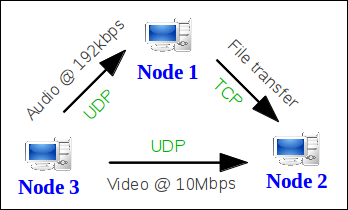
Figure 1. simple experiment scenario using three WI-FI nodes.
The experiment shown above, also called Iperf Sender Receiver (ISR) experiment , is realized using the iperf measurement tool which is a commonly used in network testing application. The iperf tool has a number of output formats instrumented for different uses. For example when iperf is used for TCP streaming, throughput information is displayed and when used for UDP streaming, jitter and packet loss information are displayed to the end user. Therefore an application can instrument more than one output to the user and in the context of OMF, they are refereed to as measurement points (MP). For this experiment scenario, transfer, jitter, and loss measurement points are used. A graphical view of experiment resource grouping is shown in figure 2.
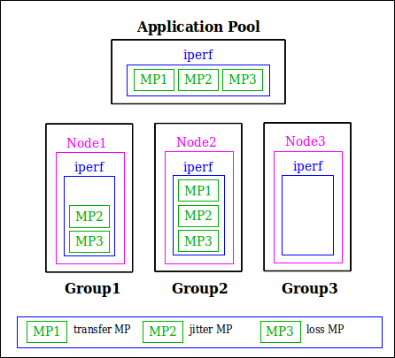
Figure 2. Experiment resource grouping of the experiment scenario. Note that Node3 does not have measurement points since it only streams UDP packets.
Next we look at how experiment is defined in the experiment definition tool. The ISR experiment, defined previously, is used here to illustrate tool's usage. From an experimenter point of view, there are two ways of defining an experiment. These are defining new experiment and defining from a saved configuration file.
Click the Start New Configuration link to start defining a new experiment. The first stage of experiment definition is experiment abstract. Here the experimenter can give a high level information about the experiment such as project name, experiment name, title, author, contact information, summary, and duration. Figure 3 shows the experiment abstract of the ISR experiment.
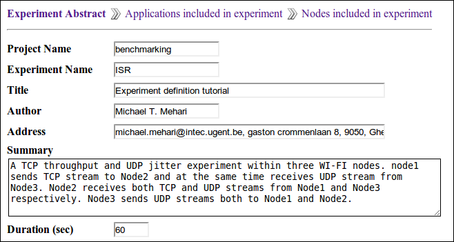
Figure 3. Experiment abstract definition of ISR experiment.
The next step is application definition. Here we create the application pool containing all applications that will be used in the experiment. Figure 4 shows the iperf application from ISR experiment application pool.
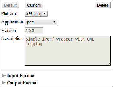
Figure 4. iperf application defined inside the application pool.
The last step in experiment definition tool is binding applications from the pool to different nodes of the wireless testbed. It involves platform specific node selection from testbed layout, interface configuration of group of nodes, and finally binding applications to nodes. Application binding involves a number of steps which are application selection, optional output instrumentation, input parameter configuration, and application timeline definition. Figure 5 shows the node configuration section (only shown for group Node1) of the ISR experiment.
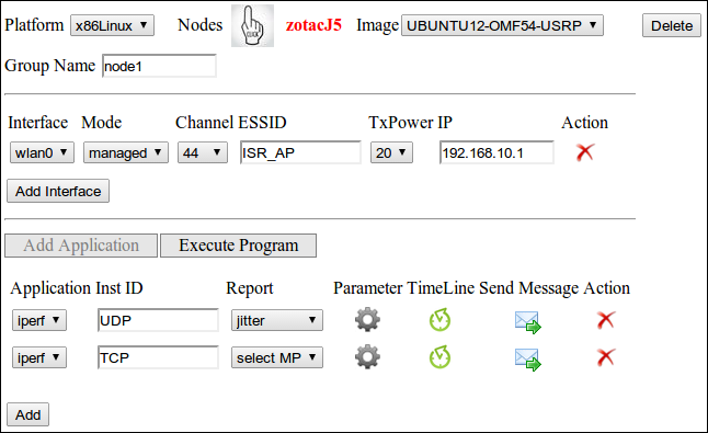
Figure 5. Experiment node configuration of ISR experiment.
Finally after finish configuring the experiment definition, we save it to a configuration package (name it ISR) composed of three files. These are XML configuration file (ISR.xml), OEDL (OMF Experiment Description Language) file (ISR.rb), and a network simulation file (ISR.ns) containing all configuration setting to be used inside emulab framework [2]. We explain the content of the XML configuration file in this section but the rest two files are explained on a separate page.
In CREW, XML is used as a configuration format for experiment descriptions and the XML configuration of the experiment definition in particular is a subset of the CREW common data format. An overview of the XML configuration of the ISR experiment is shown in figure 6.
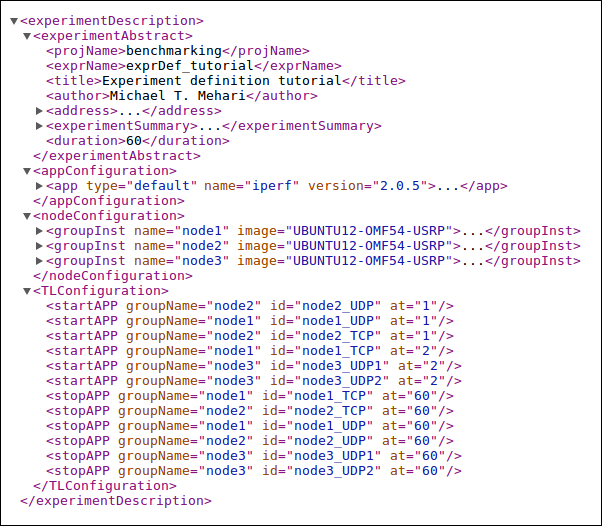
Figure 6. Excerpt from ISR experiment XML configuration file
Defining an experiment from a saved configuration file
For the experimenter, defining everything from scratch might be time consuming. An experimenter can use an existing configuration file or customize it according to his need. Reconfiguration is done first by downloading the configuration file (look CREW repository, background environments section in CREW portal) and then loading it on the "Load/Configure Experiment" section of the experiment definition tool. Finally, start reconfiguration and save it after finish modification.
[1]. Thierry Rakotoarivelo, Guillaume Jourjon, Maximilian Ott, and Ivan Seskar, ”OMF: A Control and Management Framework for Networking Testbeds.”
Configure parameters, provision and run experiments
Tool Location (OpenVPN required): http://ec.wilab2.ilabt.iminds.be/CREW_BM/BM_tools/exprExec.html
Experiment Execution Tool
Recall at the end of CREW experiment definition tool, we end up with a tar package containing three different files. The first file, ISR.xml, is an XML experiment description file for the ISR experiment. The second file generated, ISR.rb, is an experiment description of the type OEDL (OMF Experiment Description Language) and the last file generated, ISR.ns, is a network simulation file containing all configuration settings to be used inside emulab framework. Current implementation of the CREW experiment execution tool only works on top of OMF (cOntrol and Management Framework) testbeds. But it is designed to be versatile and work with different testbeds having their own management and control framework. The tool interacts with the testbed using a specific API designed for the testbed. Thus working on a different testbed with a different framework only relies on the availability of interfacing APIs and minor change on the framework itself.
Coming back to what was left at the end of the experiment definition tool, we start this section by using the two files generated (i.e. ISR.rb and ISR.ns). Details of the ISR.rb file and OEDL language are described on a separate page. However, to have a deeper understanding of the language details, one can study OEDL 5.4.
We start by definining the experiment topology on the emulab framework [1] using the NS file ISR.ns. Tutorial about creating your first experiment on the emulab framework and explanation of the NS file follows this page. After finish defining your topology and swapping in your experiment in the emulab framework, start the experiment execution tool. The experiment execution tool allows experimenters load an experiment description, configure parameters, schedule, and finally start an experiment. Figure 1 shows the front view of the experiment execution tool after the OEDL file (i.e. ISR.rb) is loaded.
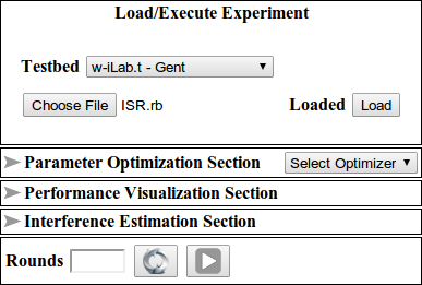
Figure 1. Experiment execution tool at glance.
After loading the file, four different sections are automatically are populated and each section performs a specific task.
- Parameter Optimization Section configures single/multi dimensional optimizer that either maximizes or minimizes an objective performance.
- Performance Visualization Section configures parameters to be visualized during experiment execution.
- Interference Estimation Section configures the pre/post interference estimation of experiments and detect unwanted wireless interference that could influence the experiment.
- Experiment Rounds section configures the number of identical runs an experiment is executed.
Recall the scenario of ISR experiment where Node 1 performs a file transfer to Node 2 while at the same time listening to a high quality (192kbps) radio channel from Node 3 and Node 2 is watching a 10Mbps movie stream from Node 3.
Now starting from this basic configuration, let us say we want to know how large the video bandwidth from Node 3 to Node 2 can increase so that we see a high definition movie at the highest possible quality. This is an optimization problem and next we see how to deal with such a problem using the experiment execution tool.
- Select IVuC optimizer from the Parameter Optimization section and click the text on the left side to reveal its content.
- Select Node3_UDP2_bandwidth as design space parameter located at the end of the Tune list.
- Start from 10,000,000 bps using step size 2,000,000 bps and reduction rate of 0.5. The optimizer either stops once the step size is reduced to 100,000 bps or when search parameter exceeds 20,000,000 bps.
- In the objective variables subsection, configure two variables to calculate the sending and receiving bandwidth using the aggregation AVG.[ Note: Click the plus icon on the right hand corner to add extra variables]
- Define your objective function as a ratio of the two variables (i.e. (8*x1)/x2) defined previously and select the condition less than with a stopping criteria 0.95 (i.e. (8*x1)/x2 < 0.95 => Stop when 8*x1 < 0.95*x2). [ Note: The reason 8 is multiplied to x1 variable is because iperf reports bandwidth in byte/sec].
Figure 2 shows the configuration details of parameter optimization section.
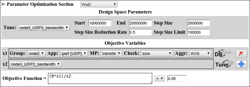
Figure 2. IVuC optimizer configuration for the ISR experiment.
The next thing we do is configure the performance visualization section where we define parameters to be visualized during experiment execution. For this exercise, we visualize the UDP and TCP bandwidth performance at Node2 coming from Node3 and Node1 respectively. As the wireless medium is shared among all Nodes, the UDP bandwidth stream from Node3 is affected by the TCP bandwidth stream from Node1 and visualizing these two parameters reveal this fact. Figure 3 shows the configuration detail of performance visualization section.
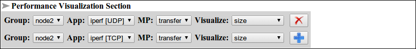
Figure 3. Performance visualization configuration for the ISR experiment
After that, we can enable interference estimation and check for possible pre and post experiment interferences. This is one way of detecting outlier experiments as there is a higher possibility for experiments to be interfered if the environment before and after their execution is interfered. For now, we skip this section. Similar to the experiment definition tool, execution configuration settings can be saved to a file. Click the button  to update the execution configuration into the OEDL file and later reloading the file starts the experiment execution page pre configured. Finally, set the number of experiment rounds to one and click on the button
  .
.
Once the experiment has started, the first thing we see is a log screen populated with debug information. The debug information contains high level information about the experiment such as defined properties, experiment ID, events triggered, and a lot more. The log screen view being an important interaction tool to the experimenter, there is also a second view called the graph screen view. To switch to the graph screen view, click the notebook icon  from the experimentation screen. The graph screen view displays parameters that were defined in the performance visualization section (see above) as a function of time. For the ISR experiment, the UDP and TCP bandwidth plot as a function of time from node3 and node1 are displayed respectively. Figure 4 shows the graph screen view of the ISR experiment.
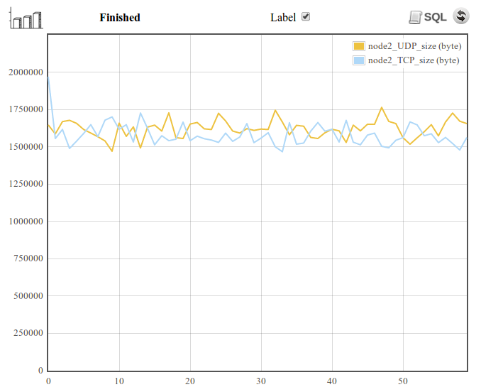
Figure 4. A glance at the graph screen view from experimentation screen.
From the above figure, we note a couple of things. Top on the left, there is the graph icon which triggers the debug information view up on clicking. Next is the experiment status (i.e. Scheduled, Running, Finished) indicator. The label check box turns the label ON and OFF. Execution of SQL statements is allowed after the experiment has stopped running. SQL statements are written in the log file viewer by which switching to this view, writing your SQL statements and pressing the icon  executes your statements. Finally the UDP and TCP bandwidth as a function of time are plotted and it also indicates an equal bandwidth share between both applications. Not shown on the figure but also found on the experimentation screen are parameter settings, objective value, correlation matrix table, and experiment run count.
Following the whole experimentation process, we see the ObjFx. Value (i.e. (8*x1)/x2) starts around 1 and decreases beyond 0.95 which triggers the second experimentation cycle. The optimization process carries on and stops when step size of Node3_UDP2_bandwidth reaches 100,000 bps. The whole process takes around 11 minutes under normal condition. The IVuC optimizer locates an optimal bandwidth of 14.125 Mbps UDP traffic from Node3 to Node2. Therefore the highest bit rate a movie can be streamed is at 14.125 Mbps.
Finally, the experimenter has the option to save experiment traces and later perform post processing on the stored data. CREW also incorporates a post processing tool to facilitate benchmarking and result analysis. The aim of this tool is to make comparison of different experiments through graph plots and performance scores. A performance score can be an objective or a subjective indicator calculated from a number of experiment metrics. The experiments themselves doesn't need to be conducted on a single testbed or with in a specific time bound, as long as experiment scenarios (aka experiment meta data) fit in the same context. Thus an experiment once conducted can be re-executed at a latter time in the same testbed or executed on a different testbed and conduct perform comparison of the two solutions.
For this tutorial save the experiment (i.e. press the Save experiment result button) by giving a name (e.g. Solution_one) and start post processing on the saved data using the benchmarking and result analysis tool. Please be reminded that only selected experiment runs are saved to a file and you should tick the check box next to each experiment run that you want to save.
List of optimizers explained
Experiment optimization is the heart of the CREW experiment execution tool. The efficiency of an experiment execution tool mostly depends on how it optimizes the different experiments to come and how fast it converges to the optimum. However, due a variety of problems in the real world, coming up with a single optimizer solution is almost impossible. The normal way of operation is to categorize similar problems into groups and apply unique optimizers to each one of them. To this end, the experiment execution tool defines a couple of optimizers which are fine tuned to the needs of most experimenters. Thus this paper explains the working principle of each optimizer supported in the experiment execution tool.
Step Size Reduction until Condition (SSRuC) optimizer
SSRuC is a single parameter optimizer aimed at problems which show local optimum or local minimum in the vicinity of the search parameter. Such kinds of problems are approximately described using two monotonically increasing and decreasing functions from either side of the optimum point. Figure 1 explains the problem graphically.
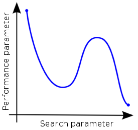
Figure 1. An example showing two local optimas with monotonic functions on either side of the optimum points
SSRuC tackles such problems using the incremental search algorithm approach [1]. Five parameters are passed to the optimizer. These are the starting, ending, step size of the search parameter, the step size reduction rate and the step size limit used as a stopping criteria by the optimizer. The optimizer starts by dividing the search parameter width into fixed intervals and performs unique experiment at each interval. For each experiment, measurement results are collected and performance parameters are computed. Next, a local maximum or local minimum is selected from performance parameters depending on the optimization context. If the optimization context is "maximization", we take the highest score value whereas for "minimization" context, we take the lowest score value. After that, a second experimentation cycle starts this time with a smaller search parameter width and step size. The experimentation cycle continues until the search parameter step size lowers below the limit. Figure 2 shows the different steps involved.
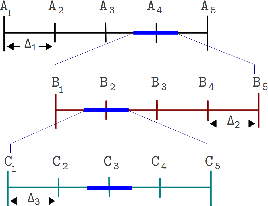
Figure 2. The different steps involved in an SSRuC optimizer over the search parameter width A1 to A5
Figure 2 shows the SSRuC optimizer in a three level experimentation cycle. In the first cycle, five unique experiments are conducted out of which the fourth experiment (experiment A4 ) is selected. The second experimentation cycle works in the neighborhood of A4 with a reduced step size ?2 . This cycle again conducts 5 unique experiments out of which the second experiment (experiment B2 ) is selected. The last experimentation cycle finally conducts 5 unique experiments from which the third experiment (experiment C3) is selected and treated as the optimized value of the parameter.
Increase Value until Condition (IVuC)
IVuC optimizer is designed to solve problems which show either increasing or decreasing performance along the design parameter. A typical example is described in the experiment execution tool where video bandwidth parameter was optimized for a three node Wi-Fi experiment scenario. Datagram error rate was set as a performance parameter and the highest bandwidth was searched limited to 10% datagram error rate and below.
The algorithm used by IVuC optimizer is similar to the SSRuC optimizer in such a way that both rely on incremental searching. However, the main difference between the two is that the SSRuC optimizer performs a complete experimentation cycle before locating the local optimum value whereas the IVuC optimizer performs a local optimum performance check after the end of each experiment. Later on, both approaches refine their searching parameter range and restart the optimization process to further tune the search parameter. Figure 3 shows the different steps involved in IVuC optimizer.
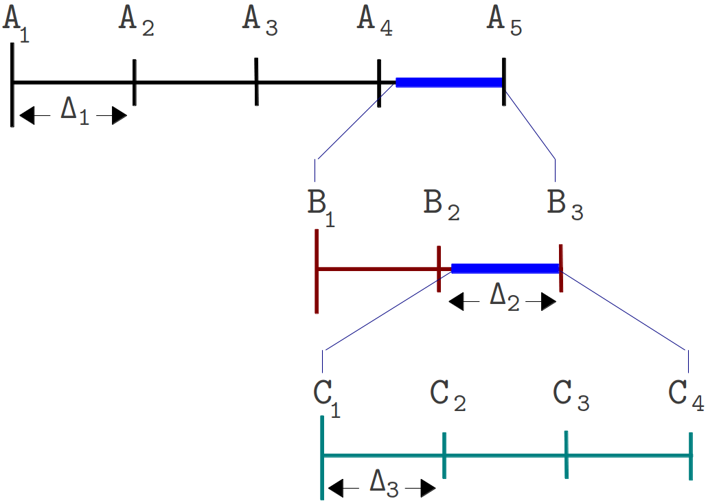
Figure 3. The different steps involved in an IVuC optimizer over the search parameter width A1 to A5
From figure 3, we see the three experimentation cycles each with five, three, and four unique experiments respectively. At the end of each experimentation cycle, performance parameter drops below threshold and that triggers the next experimentation cycle. At the end of the third experimentation cycle, a prospective step size ?4 was checked and found below threshold, making C4 the optimal solution.
Unlike SSRuC and IVuC, SUMO optimizer works on multiple design parameters and multiple design objectives. It is targeted to achieve accurate models of a computationally intensive problem using reduced datasets. SUMO manages the optimization process starting from a given dataset (i.e. initial samples + outputs) and generates a surrogate model. The surrogate model approximates the dataset over the continuous design space range. Next it predicts the next design space element from the constructed Surrogate model to further meet the optimization’s objective. Depending on the user’s configuration, the optimization process iterates until conditions are met.
The SUMO optimizer is made availabe as a MATLAB toolbox and works as a complete optimization tool. It bundles both the control and optimization functions together where the control function sitting at the highest level manages the optimization process with specific user inputs. Figure 4 shows SUMO toolbox in a nutshell highlighting the control and optimization functions together.
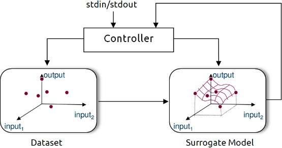
Figure 4. Out of the box SUMO toolbox in a nutshell view
In the context of CREW benchmarking tools, the aim is to use SUMO toolbox as a standalone optimizer and put it inside the experimentation framework. This means starting from out of the box SUMO toolbox, the loop is broken, the control function is removed and clear input/output interfaces are created to interact with the controlling framework. Figure 5 shows how modified SUMO toolbox is integrated in the wireless testbed.
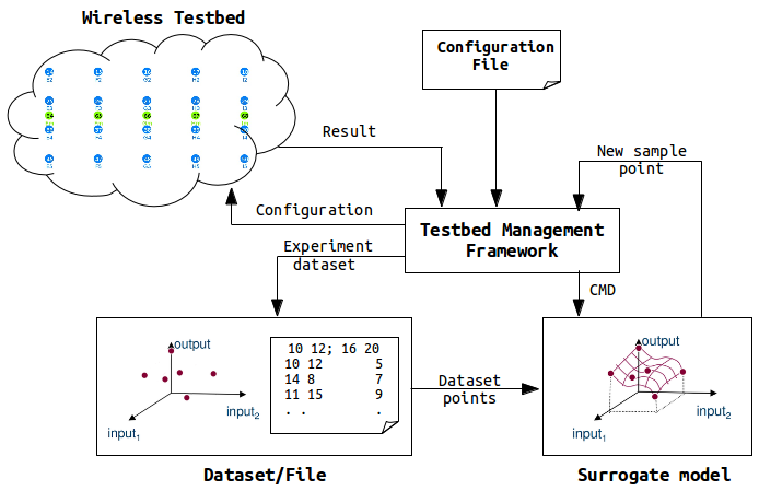
Figure 5. Integration of SUMO toolbox in a wireless testbed
The testbed management framework in the above figure controls the optimization procdess and starts by executing a configuration file. The controller pases configurations and control commands to the wireless nodes and measurement results are send back to the controller. After executing a number of experiments, the controller starts the SUMO toolbox supplying the experiment dataset which has been executed so far. The SUMO toolbox creates a surrogate model from the dataset and returns the next sample point to the controller. The controller again executes a new experiment with the newest sample point and generates a new dataset. Next the controller calls the SUMO toolbox again sending the dataset (i.e. one more added). The SUMO toolbox creates a more accurate surrogate model with the addition of one dataset. It sends back a new sample point to the controller and the optimization continues until a condition is met. It should be understood, however, that operation of the customized SUMO toolbox has not changed at all except addition of a number of blocks.
Having said about its operation, an example of wireless press conference optimization using customized SUMO toolbox is located on this link.
[1]. Jaan Kiusalaas, ”Numerical Methods in Engineering with MATLAB” Cambridge University Press, 01 Aug 2005, pp 144-146.
OEDL explained
This section provides a detailed description of the experiment description file, ISR.rb, that was created during the hands on tutorial on experiment definition tool. It mainly focus on introducing the OEDL language, the specific language constructs used inside ISR.rb file, how it is mapped to the XML experiment description file, and finally a few words on the tools OEDL language capability.
OEDL (OMF Experiment Description Language) is a Ruby based language along with its specific commands and statements. As a new user, it is not must to know the Ruby programming language. And with a simple introduction on the language, one can start writing a fully functional Experiment Description (ED) file. Any ED file written in OEDL is composed of two parts
- Resource Requirements and Configuration: this part enumerates the different resources that are required by the experiment, and describes the different configuration to be applied.
- Task Description: this part is essentially a state-machine, which enumerates the different tasks to be performed using the requested resources.
This way of looking an ED file is a generic approach and basis for learning the OEDL language. But specific to this tutorial we take a different approach and further divide content of an ED file into three sections.
Application Definition section
This section of ED file, all application resources taking part in the experiment are defined. Each application defines specific properties like input parameters, measurement points, and application specific binaries. Figure 1 shows an excerpt of the application definition from ISR.rb file.
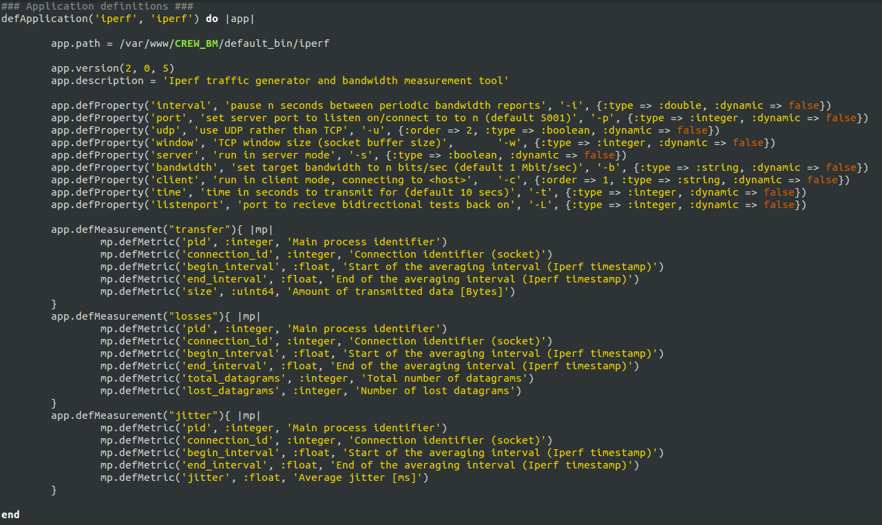
Figure 1. excerpt of ISR.rb application definition
From figure 1, we see a number of OEDL specific constructs. The defApplication command is used to define a new application. Such defined application can be used in any group of nodes as required. The defProperty command defines an experiment property or an application property. Experiment property is a variable definition that can be used anywhere inside the OEDL code. For example node1_UDP_server and node1_UDP_udp are two property definitions inside ISR.rb file. Application property on the other hand is defined inside an application and can only be accessed after the application is added. For example interval, port, udp, and others are application properties of iperf program. Next is the defMeasurement command used to define a single Measurement Point (MP) inside an application definition. Finally the defMetric command defines different output formats for the given MP.
Group Definition section
In the group definition, a group of nodes are defined and combined with the applications defined earlier. Figure 2 shows an excerpt of ISR.rb file group definition only for Node1.
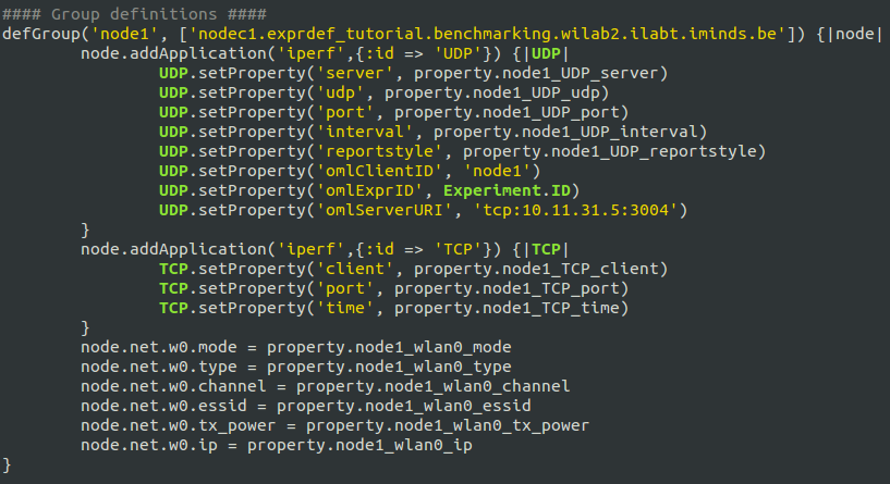
Figure 2. excerpt from iperf group definition in ISR.rb file
In this section, a number of OEDL specific constructs are used. The first one is defGroup which is used to define group of nodes. Here only nodeC1 from the testbed is defined inside the group Node1. addApplication is the second command used and it adds application into the group of nodes from the application pool. Since it is possible to add a number of identical applications with in a single group, it is good practice to give unique IDs to each added application. For the Node1 group, two iperf applications are added with IDs TCP and UDP. setProperty command is used to set values to different input parameters of the application added. Finally node specific interface configuration is handled by resource path constructs. For the Node1 group mode, type, channel, essid, tx_power, and ip configurations are set accordingly.
Timeline Definition section
The timeline definition defines the starting and stopping moments of each defined applications with in each group of nodes. Figure 3 shows an excerpt of ISR.rb file timeline definition.
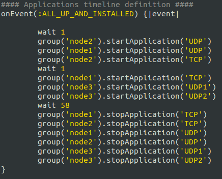
Figure 3. excerpt from iperf timeline definition in ISR.rb file
Inside OEDL language, events play a huge role. An Event is a physical occurrence of a certain condition and an event handler performs a specific task when the event is triggered. ALL_UP_AND_INSTALLED event handler shown in figure 3, for example, is fired when all the resources in your experiment are requested and reserved. The wait command pauses the execution for the specified amount of seconds. Starting and stopping of application instances are executed by the commandstartApplication and stopApplication respectively. Application IDs are used to start and stop specific applications. For example group('node1').startApplication('UDP') refers to the application iperf from node1 group with ID UDP.
So far we walk you through the default OEDL constructs that are used throughout the ISR.rb file. It is also possible to define custom OEDL constructs and one such use is custom event definition. We used custom event definition in our ISR.rb file to check if all applications are stopped. If so we trigger the EXPERIMENT_DONE event and end the experiment execution. Figure 4 shows the custom event definition used inside ISR.rb file.
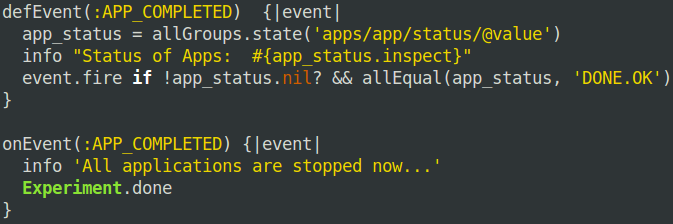
Figure 4. custom event definition section in ISR.rb file
We create a custom event using the command defEvent. By default custom defined events are checked every five seconds for possible event triggering. Inside the event definition, we wait until all applications are finished and fire the event handler afterwards. The event handler is defined following the onEvent commandpassing name of the event definition APP_COMPLETED. Finally when the event is triggered, the handler calls the EXPERIMENT_DONE method which stops the experiment execution and releases all allocated resources.
Mapping OEDL to XML experiment description
Recall from experiment definition tool section that an experimenter passes three steps to finish configuring its experiment and produce XML, OEDL, and ns files. It is hidden to the experimenter however that an OEDL file is generated from the XML file. During the making process of configuration package, an XML template is first produced out of which the OEDL file is constructed.
The mapping of OEDL to XML is straight forward. It follows a one to one mapping except rearrangement of text. The following three figures show a graphical mapping of XML to OEDL on application definition, group definition, and timeline definition sections accordingly.
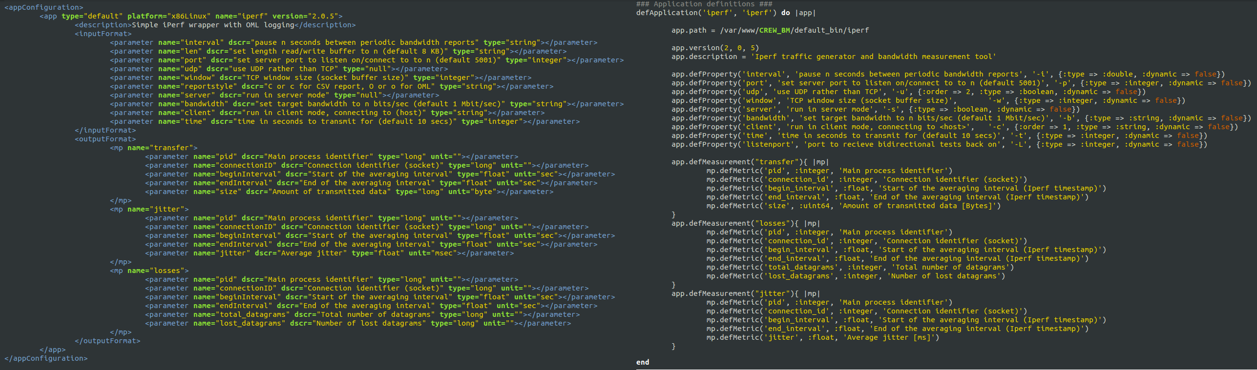
Figure 5. XML to OEDL application definition mapping inside ISR.rb file
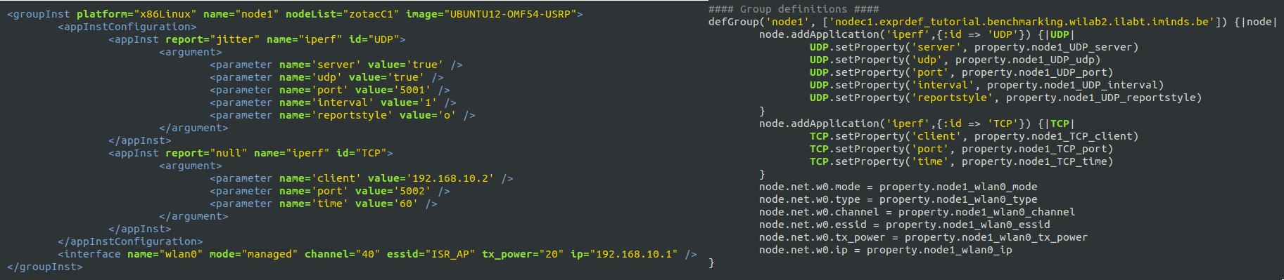
Figure 6. XML to OEDL group definition mapping inside ISR.rb file
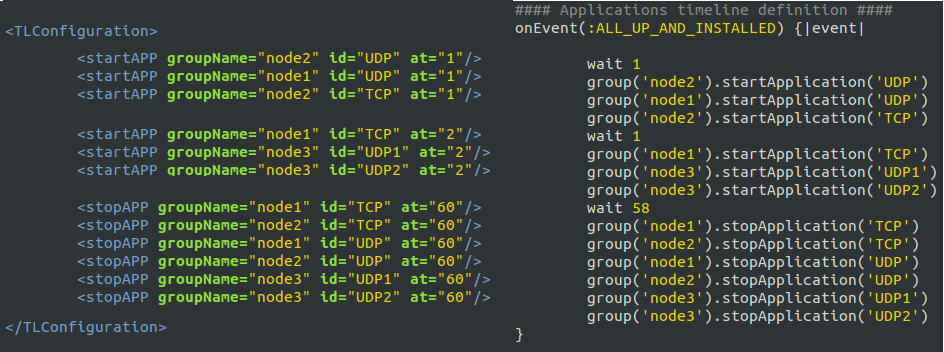
Figure 7. XML to OEDL timeline definition mapping inside ISR.rb file
Wireless press conference optimization using SUMO toolbox
Problem Statement
A wireless press conference scenario comprises of a wireless speaker broadcasting audio over the air and a wireless microphone at the listner end playing the audio stream. This type of wireless network is gaining attention specially in a multi-lingual conferencing room where the speaker's voice is translated into different language streams and broadcasted to each listner where they select any language they want to hear the translated version. However the wireless medium is a shared medium and it is possible to be interfered by external sources and we want to optimize the design parameters which gives the best audio quality. Moreover, we also want to reduce the transmission exposure which is a direct measure of electromagnetic radiation. Transmission exposure is gaining attention these days related to health issues and regulatory bodies are setting limits on maximum allowable radiation levels. Thus our second objective is to search design parameters that lowers transmission exposure of the wireless speaker exposed on each listner. For this tutorial, two design parameters of the wireless press conference are selected (i.e. transmit channel and transmit power) and we optimize these parameters inorder to increase the audio quality and decrease transmission exposure.
Experiment scenario
The experiment is composed of one speaker and 5 listeners making the Solution Under Test (SUT) and one public access point creating a background interference. The public access point is connected to three WI-FI users and provides a streaming video service at the time. Figure 1 shows the experiment scenario.
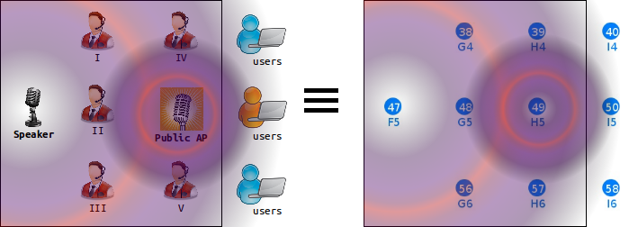
Figure 1. Experiment scenario of 5 listners, 1 speaker , 1 public access point, and 3 users.
On the left hand side, the realistic press conference scenario is shown. On the right hand side, the experimentation scenario as seen on the w.ilab.t zwijnaarde testbed [1] is shown. The horizontal and vertical distances between consecutive nodes is 6m and 3.6m respectively. All listener nodes (i.e. 38, 39, 48, 56, and 57) are associated to the speaker access point (i.e. node 47). Background interference is created by the public access point (i.e. node 49) transmitting on two WI-FI channels (i.e. 1 and 13) at 2.4Ghz ISM band.
The wireless speaker, configured on a particular transmit channel and transmit power, broadcasts a 10 second WI-FI audio stream and each listener calculates the average audio quality within the time frame. The wireless speaker at the end of its speech averages the overall audio quality from all listeners and makes a decision on its next best configuration. The wireless speaker using its newest configuration again repeats the experiment and produces a second newest configuration. This way the optimization process continues iterating until conditions are met.
The public access point on the other side transmits a 10 Mbps continuous UDP stream on both channels (i.e. channel 1 and 13) generated using iperf [2] application. In the presence of interference, audio quality gets degraded and the wireless speaker noticing this effect (i.e. lower audio quality) has two options to correct it. Either increase the transmission power or change the transmission channel. Making the first option is unlikely because it increases the transmission exposure. Changing the transmission channel also has limitations; the problem of overlapping channels interference [3]. Overlapping channels interference results in quality degradation much worse than identical channel interference. In identical channel interference, both transmitters apply CSMA-CA algorithm and collision is unlikely to happen. However in overlapping channels interference, transmitters don’t see each other and collision likely happens.
Two fold optimization
As was explained previously, we want to optimize the design parameters that brings an increased audio quality and decreased transmission exposure. A straight forward solution is to perform unique experiments at each design parameter combinations also known as exhaustive searching and locate the optimum design parameters which gives the highest combined objective (i.e. audio quality + transmission exposure).
Audio quality objective
In the earlier telephony system, Mean Opinion Score (MOS) was used for testing audio quality out of a 1 to 5 scale (i.e. 1 for the worst and 5 for the best quality). MOS is a subjective quality measure that no two people give the same score. However due to recent demands in Quality of Service (QoS), subjective scores are replaced by objective scores for the reason of standardization. Moreover, the earlier telephony system is now replaced by the more advanced Internet Protocol (IP) driven backbones where Voice over IP (VoIP) service becomes the prefered method of audio transportation.
In a VoIP application, audio quality can be affected by a number of factors. Amongst all packet loss, jitter, and latency take the most part. An objective quality measure based on these parameters is standardized as ITU-T PESQ P.862. A mapping of PESQ score to MOS scale is presented in [4]. Here packet loss, jitter, and latency are measured for a number of VOIP packets arriving at the receiver end. Averaging over arrived number of packets, jitter and latency are combined to form an effective latency which also considers protocol latencies. Finally, the packet loss is combined to effective latency in a scale of 0 to 100 called the R scale. Finally the R scale is mapped to 1 to 5 scale and MOS score is generated. Figure 2 shows the pseudo code excerpt of MOS calculation.
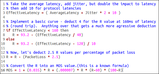
Figure 2. MOS score calculation code excerpt
Tranmission exposure objective
Transmission exposure is a direct measure of the electric-field strength caused by a transmitter. In [5] an in depth calculation of transmission exposure is presented. Exposure at a certain location is a combined measure of radiated power, transmitted frequency and path loss. Now a days regulatory bodies are setting maximum allowable exposure limits in urban areas. For example Brussels, captial city of Belgium, sets transmission exposure limit to 3v/m.
Characterizing the exposure model requires calculation of the path loss model specific to the experimentation site. The experimentation site at our testbed has a reference path loss of 47.19 dB at 1 meter and path loss exponent 2.65. Having this measurement, transmission exposure is calculated for each participating nodes and later average the sum over the number of nodes. Figure 3 shows the average exposure model.
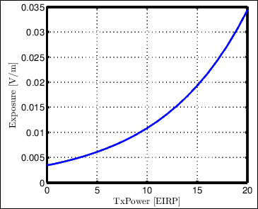
Figure 3. Average transmission exposure
Exhaustive searching optimization
The exhaustive searching optimization performs in total 13 channels x 20 TxPower = 260 experiments. Figure 4 and 5 shows performance output of the exhaustive searching optimization.
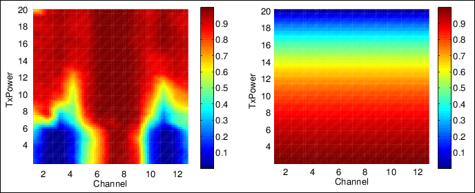
Figure 4. Audio quality and exposure global accurate model with background interference at channels 1 and 13
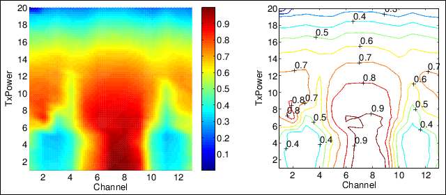
Figure 5. Dual objective and contour global accurate model with background interference at channels 1 and 13
The dual objective model shown in figure 5 is combined from the audio quality and exposure models shown in figure 4. Looking into the audio quality model, areas with a higher transmission power have good performance in general. However, there is an area on the non-interfered channel (i.e. 6 to 8), where there is a sudden jump in performance as TxPower increases from 4 dBm to 8 dBm. This area is of interest to us where higher audio quality and lower transmission exposure are seen. Indeed this is shown as a dark red region in the dual objective global accurate model.
Another aspect to look is the area where worst performance is recorded. Look again on the left side of figure 5 between channels 2 to 4, 10 to 12 and TxPower 1 to 7. Interestingly, this region is not located on channels where background interference is applied on but on its neighboring channels. This is due to the fact that the speaker and interferer nodes apply CSMA-CA algorithm on identical channel but not on neighboring channels which results in worst performance [3].
Note: TODO
Click the different areas on figure 4 to hear the audio quality when streamed at the specific design parameters
SUMO toolbox optimization
The exhaustive searching optimization gives the global accurate model however it takes very long time to finish the experimentation. Now we apply SUMO toolbox to shorten the duration and yet achieve a very close optimum value compared to the global accurate model shown in figure 5.
Start experiment execution using the preconfigured files located at the end of this page. The optimization process starts by doing 5 initial experiments selected using Latin Hypercube Sampling (LHS) over the design parameter space. LHS selects sample points on the design space evenly and with minimum sample points it assures providing the best dynamics of the system. For each of the five intial sample points, combined objectives are calculated which forms the inital dataset. The SUMO toolbox reads the inital dataset, creates a surrogate model out of it, and provide the next sample for experimentation to be carried on. The iteration continues until the stopping criteria is met. The stopping criteria selected, at the end of every iteration, sorts the collected combined design objective in ascending order and take the last five elements. Next calculate the standard deviation of this list and stop iteration when the standard deviation falls below threshold. A threshold of 0.05 is selected such that it is twice the standard deviation of a clean repeatable experiment [6]. The idea behind choosing such criteria is that the output of a sorted experiment approaches a flat curve as the optimization reaches the optimum. And the sorted last few elements show a small standard deviation.
Three sets of experiments are conducted and the results are compared to the global accurate model interms of Performance Gain (PG) and Duration Gain (DG) metrics. figure 7 shows the plot of sorted last 5 iteration standard deviation as a function of iteration/duration gain until stopping criteria (i.e. STD_MIN < 0.05) is met.
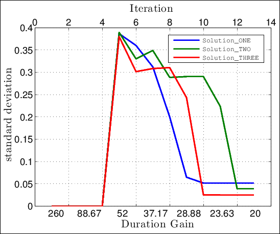
Figure 7. sorted last 5 iterations standard deviation plot
Shown in the figure above, all solutions stop execution around the 12th iteration (i.e. DG=21.5). Their perfomance gain compared to the global accurate model gives
Solution_ONE PG = [Solution optimum]/[Global accurate optimum] = -0.8261/-0.8482 = 0.9739
Solution_TWO PG = [Solution optimum]/[Global accurate optimum] = -0.8373/-0.8482 = 0.9871
Solution_THREE PG = [Solution optimum]/[Global accurate optimum] = -0.8352/-0.8482 = 0.9846
From the above results we conclude that by applying SUMO toolbox to wireless press conference problem, we improved the optimization process around 21.5 faster than the exhaustive searching optimization. And yet their performance is almost identical.
[1] http://www.ict-fire.eu/fileadmin/events/2011-09-2OpenCall/CREW/Wilabt_crewOpenCallDay.pdf
[2] Carla Schroder, ”Measure Network Performance with iperf” article published by Enterprise Networking Planet, Jan 31, 2007
[3] W. Liu, S. Keranidis, M. Mehari, J. V. Gerwen, S. Bouckaert, O. Yaron and I. Moerman, "Various Detection Techniques and Platforms for Monitoring Interference Condition in a Wireless Testbed", in LNCS of the Workshop in Measurement and Measurement Tools 2012, Aalborg, Denmark, May 2012a
[4] http://www.nessoft.com/kb/50
[5] D. Plets, W. Joseph, K. Vanhecke, L. Martens, “Exposure optimization in indoor wireless networks by heuristic network planning”
[6] M. Mehari, E. Porter, D. Deschrijver, I. Couckuyt, I. Morman, T. Dhaene, "Efficient experimentation of multi-parameter wireless network problems using SUrrogate MOdeling (SUMO) toolbox", TO COME
| Attachment | Size |
|---|---|
| audioQltyExpOptSUMO.tar | 1.9 MB |
Process and check quality
Show and compare results
Tool Location (OpenVPN required): http://ec.wilab2.ilabt.iminds.be/CREW_BM/BM_tools/exprBM.html
The benchmarking and result analysis tool is used to analyze results obtained and benchmark the solution by comparing it to other similar solutions. As the name implies, the tool provides result analysis and score calculation (aka benchmarking) services. In the result analysis part, we do a graphical comparison and performance evaluation of different experiment metrics. For example, application throughput or received datagram from two experiments can be graphically viewed and compared. In score calculation part, we do advanced mathematical analysis on a number of experiment metrics and come up with objective scores.
Benchmarking and result analysis
Most of the time the steps involved in wireless experimentation are predefined. Start by defining an experiment, execute the experiment, analyze and compare the result. This tutorial explains the last part which is result analysis and performance (aka score) comparison. In the result analysis part, different performance metrics are graphically analyzed. For example, application throughput or received datagram from two experiments can be graphically viewed and compared. In performance comparison part, we do mathematical analysis on a number of performance metrics and come up with objective scores (i.e. 1 to 10). Subjective scores can also be mapped to different regions of the objective score range (i.e. [7-10] good, [4-6] moderate, [1-3] bad) but it is beyond the scope of this tutorial.
Coming back to our tutorial, we were at the end of experiment execution tool where we saved the experiment traces into a tar ball package. Inside the tar ball package there is database.tar file containing all SQLite database files, exprSpec.txt file which holds the experiment specific details and an XML metaData.xmlfile containing the output format of the database files stored. For this tutorial we use three identical optimization problem packages (i.e. Solution_ONE,Solution_TWO, Solution_THREE). Download each package (i.e. located at the end this page) into your personal computer.
Load all tar ball packages into the result analysis and comparison tool each time by pressing the plus icon and press the load button. After loading the files, a new hyperlink START ANALYSIS appears and follow the link. Figure 1 shows front view of the tool during package loading
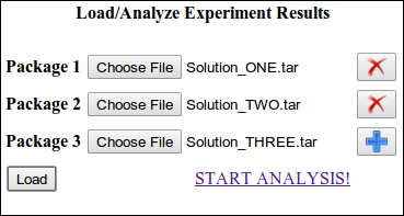
Figure 1. result analysis and performance comparison tool at glance.
Result Analysis Section
Using the result analysis section, we visualize and compare the bandwidth of Node3 as seen by Node2 for different experiment runs. Click the ADD Graph button as shown in figure 1 above. It is also possible to create as many graphs as needed. Each graph is customized by three subsections. The first is database selection. Here we select different experiment runs that we need to visualize. For this tutorial, three distinct solutions were conducted in search of the optimal bandwidth over the link Node3 to Node2. Figure 2 shows the database selection view of the ISR experiment.
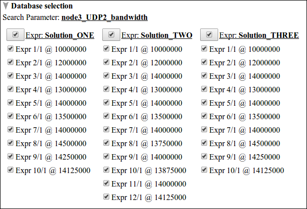
Figure 2. database selection view of the ISR experiment over three distinct solutions.
From the figure above, the search parameter node3_UDP2_bandwidth indicates the tune variable that was selected in the parameter optimization section of experiment execution tool. Moreover, The number of search parameters indicates the level of optimization carried, thus for ISR experiment it is a single parameter optimization problem. The other thing we see on the figure is solutions are grouped column wise and each experiment is listed according to experiment #, run # and specific search parameter value. For example Expr 10/1 @ 13875000 indicates experiment # 10, run # 1 and node3_UDP2_bandwidth=13875000 bit/sec. Before continuing to the other subsections, deselect all experiment databases and select only Expr 1/1 @ 10000000 from all solutions.
The second subsection, graph analysis, selects x-axis and y-axis data sets. To this end, the database meta data file is parsed into structured arrangement of groups, applications, measurement points, and metrics out of which the data sets are queried. Besides this, there are three optional selection check-boxes; AVG/STDEV, LABEL, and RANGE. AVG/STDEV is used to enable average and standard deviation plotting over selected experiments. LABEL and RANGE turns on and off plot labeling and x-axis y-axis range selection respectively.
The last subsection is custom graph analysis and it has similar function like the graph analysis subsection. Compared to the graph analysis subsection, SQL statements are used instead of parsed XML metadata to define x-axis and y-axis data sets. This gives experimenters the freedom to customize a wide of range of visualizations. Figure 3 shows graph analysis and custom graph analysis subsections of the ISR experiment. For graph analysis, begin_interval and size (i.e. bandwidth) from Node2 group, iperf_UDP application, transfer measurement point are used as x-axis and y-axis data sets respectively. For custom graph analysis, mean interval and size (i.e. bandwidth) are used as x-axis and y-axis data sets respectively.
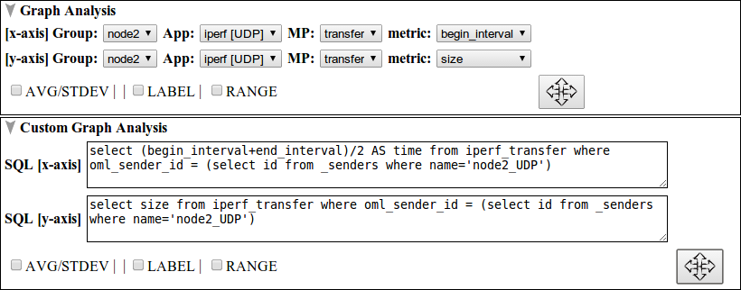
Figure 3. graph analysis and custom graph analysis subsection view.
Now click the arrow crossed button  in either of the graph analysis subsections to visualize datagram plot for the selected experiments. Figure 4 shows such a plot for six experiments.
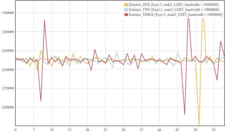
Figure 4. bandwidth vs. time plot for three identical experiments.
The first thing we see from the above figure is in each of the three experiments, Node2 reported almost identical bandwidth over the one minute time interval.Second the y-axis plot is zoomed within maximum and minimum result limits. Sometimes, however, it is interesting to see bandwidth plot over the complete y-axis range which is starting from zero up to the maximum. Click the RANGE check box and fill in 0 to 55 in the x-axis range and 0 to 1500000 in the y-axis range. Moreover, in repeated experiments one of the basic things is visualizing the average pattern of repeated experiments and see how much deviation each point has from average. Check the AVG/STDEV check-box (check the SHOW ONLY AVG/STDEV check-box if only AVG/STDEV plot is needed). Figure 5 shows the final modified plot when complete y-axis range and only AVG/STDEV plot is selected.
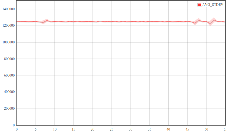
Figure 5. average bandwidth as a function of time plot from three identical experiments
Performance comparison Section
In performance comparison, a number of experiment metrics are combined and objective scores are calculated in order to compare how good or bad an experiment performs related to other experiments.
For this part of the tutorial, we create a simple score out of 100 indicating how much percent the receive bandwidth reaches and the transmit bandwidth. The higher the score the better the receive bandwidth approaches the transmit bandwidth and vise versa. Start by clicking the ADD Score button and a score calculation block is created ( Note: go further down to reach the score calculation section). A score calculation block has three subsections namely variable definition, score evaluation and database selection.
The variable definition subsection defines SQL driven variables that are used in the score evaluation process. For this tutorial, we create two variables one evaluating the average receive bandwidth and the second evaluating the transmit bandwidth. Click the plus icon twice and enter the following SQL command into the first text-area "SELECT avg(size) from iperf_transfer where oml_sender_id=(select id from _senders where name='node2_UDP')". For the second variable click the icon  to select variables from search parameters and select node3_UDP2_bandwidth.
The next subsection, score evaluation, is a simple mathematical evaluator with built in error handling functionality. Coming back to our tutorial, to simulate the percentage of receive bandwidth to transmit bandwidth, enter the string 100*(8*x1)/x2 in the score evaluation text-area ( Note: x1 is multiplied by 8 to change the unit from byte/sec to bit/sec).
Finally, database selection subsection serves the same purpose as was discussed in the result analysis section. Now press the arrow crossed button in the score evaluation subsection. Figure 6 shows the scores evaluated for the ISR experiment.
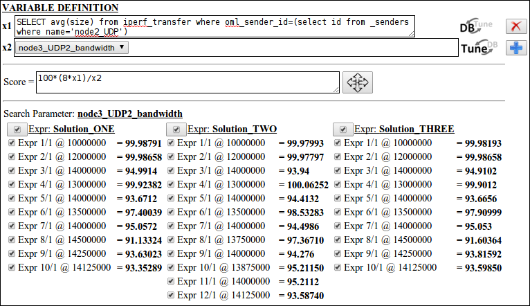
Figure 6. score evaluation section showing different configuration settings and score results for the ISR experiment.
Performance comparison is possible for identical search parameter settings among different solutions. For example comparing Expr1/1 @ 10000000 experiments from the three solutions reveals that all of them have receive bandwidth about 99.98% of the transmit bandwidth and thus they are repeatable experiments. On the other hand, the scores from any Solution show the progress of the optimization process. Recall the objective function definition (i.e. (8*x1)/x2 < 0.95 => stop when 8*x1 < 0.95*x2) in the ISR experiment such that the IVuC optimizer triggers the next experimentation cycle only when the receive bandwidth is less than 95% of the transmit bandwidth. Indeed on the figure above, search bandwidth decreases as the performance score decreases below 95%. Therefore performance scores can be used to show optimization progress and compare among different Solutions.
| Attachment | Size |
|---|---|
| Solution_ONE.tar | 380 KB |
| Solution_TWO.tar | 450 KB |
| Solution_THREE.tar | 380 KB |