Portal: advanced documentation
The sections below contain advanced information on the different CREW testbeds. For information on the benchmarking platform, please consult the section of the w-iLab.t testbed on benchmarking. You can use the menu on the left of this website to navigate through the portal. You can use the menu on the left of this website to navigate through the portal.
The information on the portal will be regularly updated as additional information and cognitive components become available.
Basic tutorial: your first experiment on w-iLab.t office testbed
Run your first experiment on w.iLab-t office testbed
!! THIS INFORMATION ONLY APPLIES TO THE w-iLab.t Office testbed. !!!
Up to date documentation on the w-iLab.t Zwijnaarde testbed can be found at http://doc.ilabt.iminds.be/ilabt-documentation/wilabfacility.html
In this basic tutorial you will learn how to run your first sensor experiment on Wilab.t. The sensor code we will use for this experiment is called RadioPerf. This application is able to send commands over the USB channel to the mote (e.g. start sending radio packets of x bytes to destination y). The mote also periodically sends reports back over the USB channel (e.g. how many packets it received, what the RSSI of the received packets was, ...). In this tutorial you will learn how to tell a sensor node to start sending packets and afterwards analyze the the result with one of the Wilab.t tools. Important note: the program and class files used in this tutorial are programmed/generated in a TinyOS environment. If you are not familiar with TinyOS, it is strongly advised to check out the TinyOS tutorials. Note that the class files are explained in tutorial 4.
Send an e-mail to  to request an OpenVPN account for the w.iLab-t testbed. Be sure to also mention your affiliation and/or project for which you want access to the testbed. We recommend downloading the VPN software from the OpenVPN website. Once you installed the software and received the necessary certificates and credentials, you should be able to connect to the w.iLab-t testbed. Make sure you run the OpenVPN software as Administrator/root !
-
Request w-iLab.t account
-
Create your first job
-
Schedule your first job
-
Analyze results
-
Visualize experiment
-
Schedule parametrized experiment
Now that you're able to connect to the w-iLab.t web interface, you can request an account on the w-iLab.t Office testbed by completing the form on the signup page. You can register for the w-iLab.t Zwijnaarde testbed by clicking "Request Account" on the w-iLab.t Zwijnaarde home page.
Once your account has been approved, you can log in to the w.iLab-t Office testbed. (The following describes your first job on the Office testbed. If instead you want to use the w.iLab-t Zwijnaarde testbed, tutorials are available at the w-iLab.t Zwijnaarde info page (10.11.31.5). After registration on the w-iLab.t Zwijnaarde home page, you should first take a look at the Emulab-OMF tutorial and reserve your nodes here. Now go to the job page to create your first job. Click the Create new job button and fill in a name and description. Click next or go to the files tab. In the files tab you must select at least one Program file and one Class File. The Program File contains the firmware that will be programmed on the sensor nodes. Sensor nodes can send messages to the w.iLab-t server which will be logged in the database. The Class Files define which messages, that are sent by the sensor node, will be logged in the database. For our first job, we will use the RadioPerf-CREW image as Program File and the RadioPerf-ReportMsg as Class File. Select them in the list on the left and click the Add>> button. 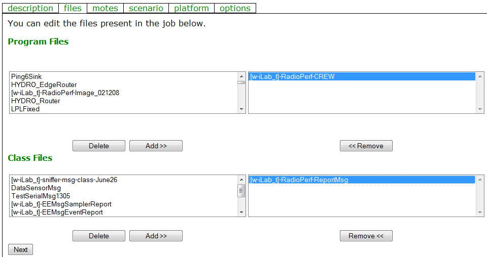 At the bottom of the files tab, it is possible to upload your own images and class files. Click Next or go to the motes tab. You can choose to run the firmware on all available sensor nodes, or pick some specific nodes out of the list. For our first experiment, we can just run the experiment on all available sensor nodes.
 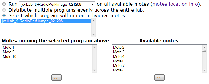 The scenario and platform tabs are not important for our first experiment, so just click the Submit button at the bottom of the page.
Now that we created our first job, we can schedule it to be executed on the testbed. On the schedule page select the job you want to execute and select a zone (part of the testbed) in which you want it to run. (Choose between 1A/1B/2A/2B/3A/3B). Now double click the first time slot where you want the experiment to start and select some consecutive blocks to determine the duration of the experiment. For this first experiment, 10 minutes should suffice. Click Schedule Job to confirm the selection. 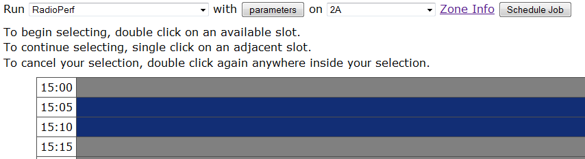
To analyze the results of your experiment (during or after), you can log in to your personal database via the user info page. You should take note of your wilab Database Name which is listing near the top of the page (this is NOT your email-adres). After clicking the phpmyadmin link, you can fill in your username and password. On the left side of the phpmyadmin page you see some general databases and one database which is named after your own user name. Click this database to see what tables it contains. For every job, there should be a table in the database (if it logged any info). Click the browse icon to see all the info your experiment has logged.
The<
toolbox page contains a list of analyzer and visualizer XML files. Select the [w-iLab_t]_Visual_RadioPerf XML file and click Start Visual to start the Java applet that will visualize your experiment. Now fill in your database user name (not email) and password. You will need to install the sun-java6-plugin to get the applet working. The applet will NOT load with the alternative OpenJDK plugin (IcedTea). The applet has been tested in both Firefox and Internet Explorer. Once the applet has finished loading, you should now see a blue circle with the sensor node id for every active node in your experiment. After some time, every node should log some info to the database and the circles should change color and now also show the estimated noise floor (ENF). In the next step we will show how we can modify the experiment by changing some parameters.
In this step we want to schedule the same job, but change some parameters so that one node will broadcast (single hop) some data packets to all nodes in its neighborhood. Therefore we go back to the
schedule page , select the job we want to run and then click the parameters button. Now look for all parameters starting with RadioPerfP. The default values can be used except for the source parameter. If we want one node to transmit packets to all other nodes (destination value 65535 equals broadcast), we must change this to the id of the transmitting node (e.g. 80 if we run the experiment on zone 2A). 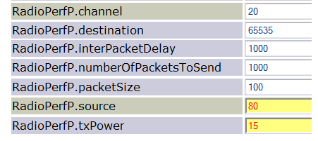 Now choose some time slots, select a zone and click the Schedule Job button. Repeat Step 6 to visualize the parametrized experiment. You should now see arrows from the sending node to all receiving nodes, with an RSSI indication next to the arrows.
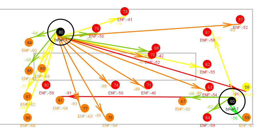
Schematic overview
Please click the thumbnail extracts below to get a full screen view of the different infrastructures. After clicking the thumbnails, click to zoom in.
The images may also be downloaded on the bottom of this page.
to zoom in.
The images may also be downloaded on the bottom of this page.
| TWIST - Berlin | w-iLab.t - Gent | Iris - Dublin | LTE-Advanced - Dresden | Log-a-tec - Ljubljana |
 Hardware overview |
 Hardware overview |
 Hardware overview |
 Hardware overview |
 Hardware overview |
 Usage overview |
 Usage overview |
 Usage overview |
 Usage overview |
 Usage overview |
| Access documentation | Access documentation | Access documentation | Access documentation | Access documentation |
| Attachment | Size |
|---|---|
| wilab-UsageOverview.png | 158.04 KB |
| wilab-HardwareOverview.png | 183.3 KB |
| TWIST-UsageOverview.png | 119.91 KB |
| TWIST-HardwareOverview.png | 114.63 KB |
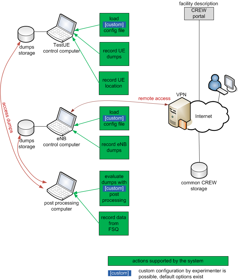
| LTE-UsageOverview.png | 88.02 KB |
| LTE-HardwareOverview.png | 188.22 KB |
| vesnaHardwareOverview_v3-s.jpg | 1.48 MB |
| IrisTestbedHardwareOverviewY2_v1.1.jpg | 402.97 KB |
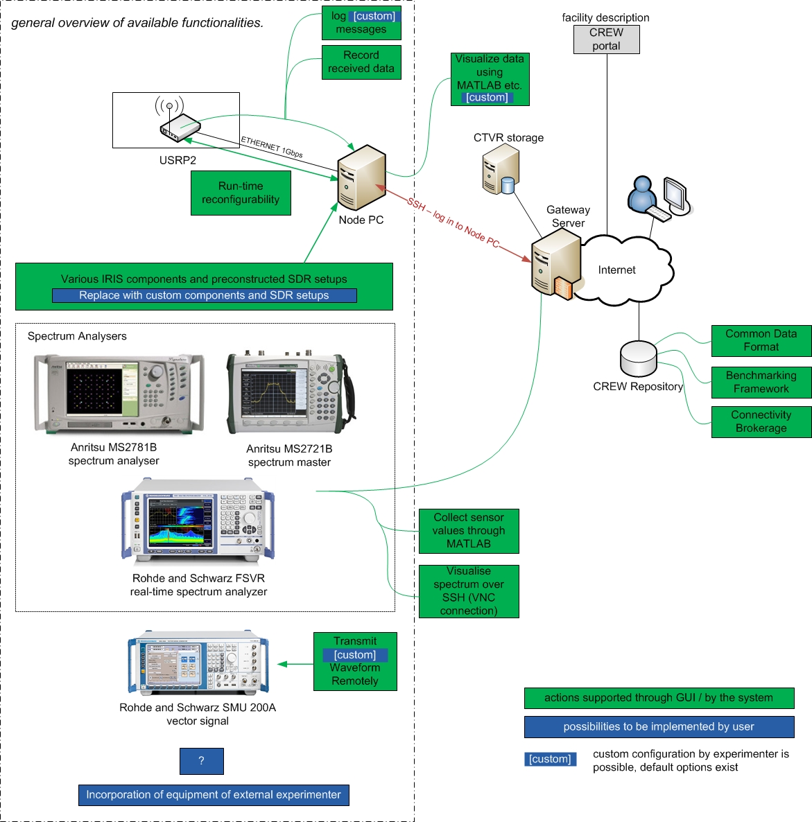
| IrisUsageOverview_v2.jpg | 482.33 KB |
IRIS documentation
The reconfigurable radio consists of a general-purpose processor software radio engine, known as IRIS (Implementing Radio in Software) and a minimal hardware frontend. IRIS can be used to create software radios that are reconfigurable in real-time.
Please use the links below to learn more about how Iris can be used.
Testbed Description
Iris is a software radio architecture that has been developed by CTVR, The Telecommunications Research Centre at TCD, Written in C++, Iris is used for constructing complex radio structures and highly reconfigurable radio networks. Its primary research application is to enable a wide range of dynamic spectrum access and cognitive radio experiments. It is a GPP-based radio architecture and uses XML documents to describe the radio structure. This testbed provides a highly flexible architecture for real-time radio reconfigurability based on intelligent observations the radio makes about its surroundings.
Each radio is constructed from fundamental building blocks called components. Each component makes up a single process or calculation that is to be carried out by the radio. For instance, a component might perform the modulation on the signal or scale the signal by a certain amount. Each component supports one or more data types and passes datasets to other components, along with some metadata such as a time stamp and sample rate. There is a data buffer between each component to ensure the data is safe, even if one component is processing data much faster than another.
All components within the radio exist inside an engine. An engine is the environment in which one or more component operates. Each engine defines its own data-flow and reconfiguration mechanisms and runs one or more of its own threads. As with components, each engine is linked by a data buffer. Iris currently features two data types, the PN Engine and the Stack Engine. The PN engine is typically used for PHY layer implementations and is designed for maximum flexibility. It has a unidirectional data flow and runs one thread per engine. The Stack Engine is designed for the implementation of the network stack architecture, where each component is a layer within the stack and runs its own thread of execution. It also has a bidirectional data flow.
Iris’s capability to reconfigure the radio on the fly lies in the controllers. A controller exists independently of any engine and runs in its own thread of execution. A controller subscribes to events within components and reconfigures parameters in other components based on the observation of these events. For instance, a controller could be set up to observe the number of packets passing through a certain component and, upon reaching a certain number of packets, change the operating frequency of the radio.
The Iris 2.0 architecture is illustrated in the following figure.
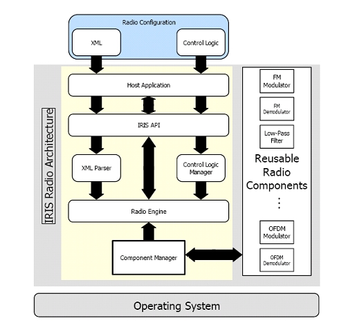
A radio is constructed and configured using XML documents. Each component is named and has its inputs, outputs and exposed parameters explicitly specified. Engines are declared and components are placed in their relevant engines. Controllers are then declared at the top of the XML document and the links between each component are declared at the end of the document.
The layout of the testbed hardware can be found here .
The testbed can be accessed directly here .
Apply for an account
Before gaining access to the Iris testbed it is essential to familiarise yourself with the Iris software. This is done through the Iris Wiki page. The Wiki gives you full instructions on how to download and install the Iris software onto your own computer as well as instructions on how to get started in using it. Use of the Wiki page requires a user account and password. These can be obtained through emailing either tallonj@tcd.ie or finnda@tcd.ie.
An overview of the Iris architecture and some of its capabilities are available here .
At this stage users will be able to performe experiments using Iris, independent of the Iris testbed, using either the simulated "channel component" or in conjunction with the USRP (1/2/N210 etc.).
Access to the Iris testbed is given out separately from access to the Wiki. This is because access to the Iris testbed is often not necessary if users have USRP hardware of their own available.
However, if remote access to the Iris testbed (after installing and trying out the Iris software) is required, details of how to obtain access to the testbed can be found here.
Remote access
The CTVR Iris testbed is currently being reconfigured. The node locations may not reflect exactly those shown in the diagram. For downtimes make sure to check the calendar.
The testbed is designed to permit fully remote access for carrying out experiments. This page provides information required to use the testbed from a remote location.
Access to the Iris testbed is achieved through the ctvr-gateway server. User login details are required to gain access to this server. These can be applied for by emailing either tallonj@tcd.ie or finnda@tcd.ie explaining the nature of the experimentation desired to be carried out within the testbed. Due to limitations in the number of nodes available applications must be handled on a case by case basis.
Once login details have been obtained
The experimenter will need to schedule an experiment.
Remote VNC Access
The experimenter will then be able to access any of the testbed nodes via VNC in the following way. Use the login details you were issued to login to ctvr-gateway.cs.tcd.ie via SSH. Once you have a terminal for this server open, SSH again onto the node you wish to access as follows:
ssh nodeuser@ctvr-node07.cs.tcd.ie
vncserver :1 -geometry 1280x900
This will create a vncserver on display 1 of node 07 and with a 1280x900 screen resolution. Once the server is running, use a VNC client to connect. In this case, we would connect to ctvr-node07.cs.tcd.ie:1. When you are finished, kill the VNC server on the testbed node as follows:
vncserver -kill :1
The following pages will be of use in setting up an experiment:
| Iris architecture overview | Iris Testbed Layout | Powering the USRPs remotely |
|---|---|---|
|
 |
 |
| Spectrum analyser remote access | First example experiment | Use fo the testbed webcam |
 |
 |
 |
Use of licensed bands
For use of wireless spectrum outside of unlicensed bands the experimenter is directed here.
| Attachment | Size |
|---|---|
| Iris Experiment.jpg | 79.47 KB |
| webcam_symbol.png | 6.43 KB |
First example experiment
The full installation instructions for iris can be found at:
https://ntrg020.cs.tcd.ie/irisv2/wiki/ExampleExperiments
The wiki contains information on how to install iris on both Windows and Linux OS.
As well as information on how to run a radio and on the test bed in general.
In this sample experiment we will run a simple radio and then adapt a component and add a controller, with a view to exploring the basic functionality of both. The steps a researcher should follow to complete the experiment are outlined below.
1. Follow the instructions outlined in the wiki to run radio, OFDMFileReadWrite.XML
2. If this radio is functioning correctly, “radio running” will appear on the command line.
3. To add a controller to the radio, we must first create an event in one of the components to which the controller can subscribe. To do this, open the shaped OFDM modulator and register an event in the constructor function.
4. Once the event is registered we must create a condition that must be satisfied for the event to be activated. To do this, open the “process” function (as this is where all the calculations are carried out) and specify a condition that activates the controller whenever, for example, 100 packets have passed through.
5. Once this has been done the controller can be made. Open the “example” controller; this gives us a template to work with.
6. Within the controller we must do two things, subscribe to the event that has been set up in the component and specify the parameter that we wish to change as well as the value we wish to change it to.
7. To change the parameter, we specify the name of the parameter as well as the component and engine that it is in. These are assigned in the “ProcessEvent” function.
8. The logic that dictates what the parameter is changed to also goes in this function.
9. Recompile all the relevant code, include the controller in the XML file and run the radio as before.
If the radio is running properly, you should see the event being triggered on the command line and the new value of the parameter in question.
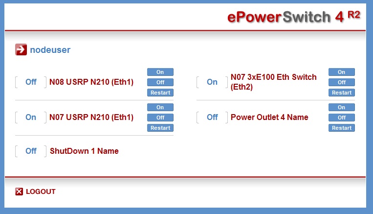
Control of the USRP remote power switches
Powering the USRPs
In the testbed we have installed two remote power switches which allow us to remotely power each of the USRPs on and off. To access the remote power switches you must first be logged into one of the testbed nodes. Details on obtaining access can be found here. These switches can be controlled through web interface.
Access the switches by navigating to
or
http://ctvr-switch02.cs.tcd.ie
in the web browser of one of the testbed nodes (again, the power switch interfaces can only be accessed from the testbed nodes). On doing so you will see a similar interface to the following:
The login details are identical to those used to access the nodes themselves. Here, you can power the USRPs for each node on and off. Please remember to power USRPs off when you have finished using them. The positioning of the different testbed nodes as well as the spectrum analyser and signal generator can be found here .
Powering the USRPs via command line/scripts
The remote switch can also be accessed via HTTP Post commands, using a tool such as curl, or equivalent calls in a script or program. Using a UNIX based system with curl installed
curl --data 'P<port>=<command>' http://nodeuser:ctvrnodepass@ctvr-switch.cs.tcd.ie/cmd.html
will alter the state of socket <port> according to <command>.
<port> choices are as follows:
For switch http://ctvr-switch.cs.tcd.ie
* 1 - Node 08 USRP N210 (ETH1)
* 2 - Node 08 USRP N210 (ETH1)
* 3 - Node 05 USRP N210 (ETH1)
* 4 - Node 06 USRP2 (ETH1)
For switch http://ctvr-switch02.cs.tcd.ie
* 1 - Currently unspecified
* 2 - Currently unspecified
* 3 - Currently unspecified
* 4 - Currently unspecified
<command> choices are:
* 0 - Switch Off
* 1 - Switch On
* t - Toggle state
* r - Restart
Commands to multiple ports can be strung together using ampersands, as per the following example:
curl --data 'P0=r&P1=r&P2=r' http://nodeuser:ctvrnodepass@ctvr-switch.cs.tcd.ie/cmd.html
| Attachment | Size |
|---|---|
| e-power switch.jpg | 63.91 KB |
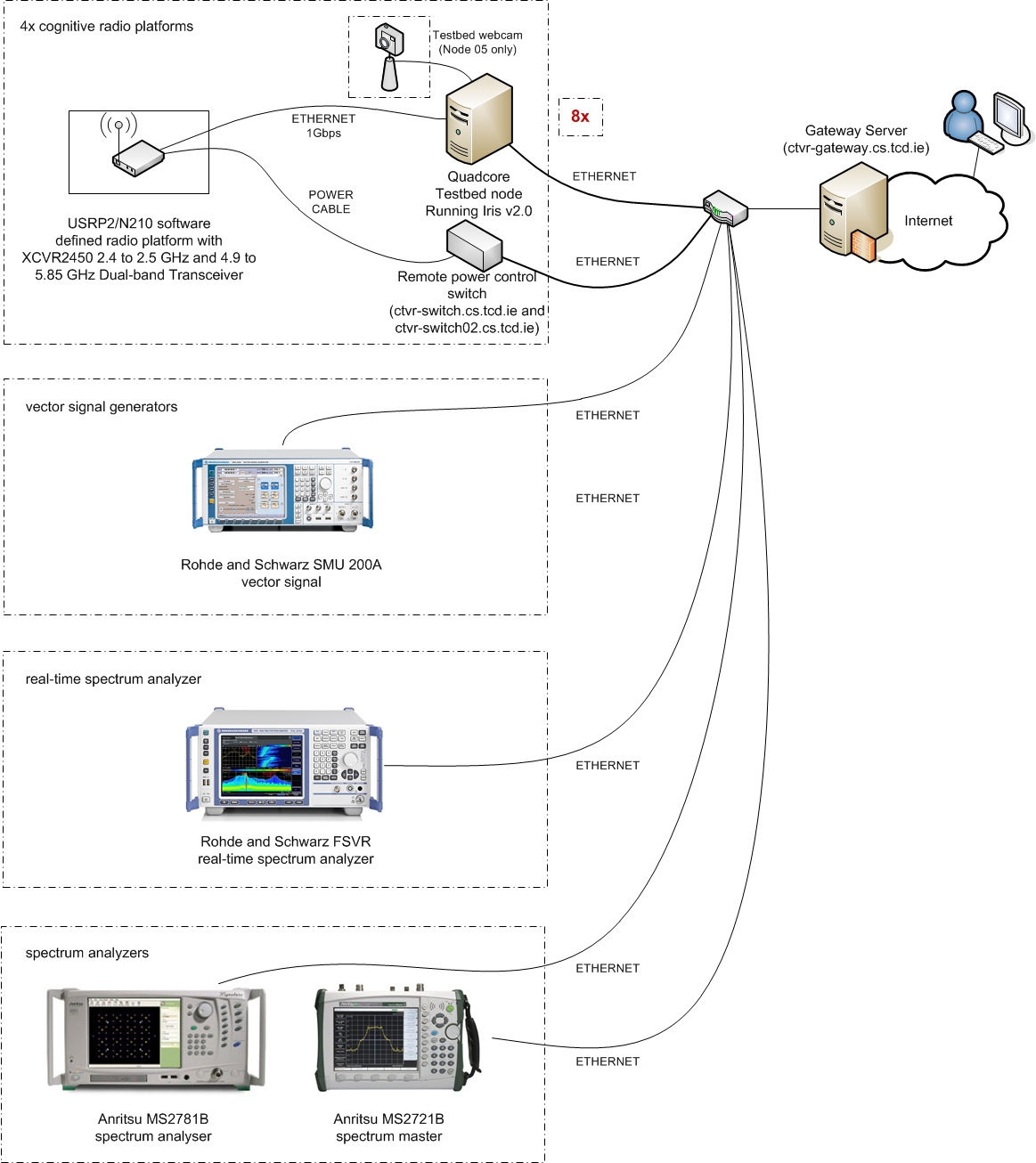
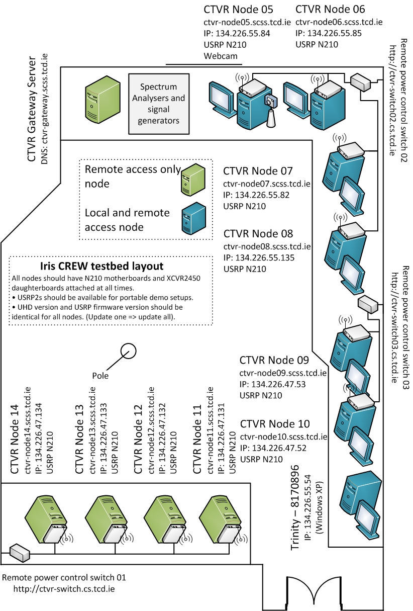
Iris Testbed Layout
The CTVR Iris testbed is currently being reconfigured. The node locations may not reflect exactly those shown in the diagram. For downtimes make sure to check the calendar.
The testbed is laid out as follows. Currently there are 8 remotely accessible Quad core machines each equipped with a USRP2/N210 and an XCVR2450 daughterboard. The USRP2s have a 24 MHz bandwidth (using Gigabit Ethernet to communicate between the USRP and the computer). The daughterboards are capable of transmitting between 2.4 and 2.5 GHz and also between 4.9 and 5.9 GHz.
The testbed diagram shows the "fixed" testbed layout; however, a some "custom" layouts may also be accommodated for specific experiments.
Additionally, before running an experiment on the testbed, experimenters must gain login details for the ctvr-gateway node, through which all of the other testbed nodes are accessed. Information on applying for login details can be found here. Experiments must also previously be scheduled on the testbed calendar, details of which can be found here.
| Attachment | Size |
|---|---|
| Testbed_Diagram_v5.2.jpg | 485.72 KB |
Iris Testbed best practices
1. Everything in the testbed has an exact place
· Each USRP and node has been assigned a table and number.
· Unused daughterboards will be placed in proper storage places.
2. Everything goes back to the exact place after any experiment that causes it to be moved.
3. Clonezilla is used on all nodes meaning that nodes will be reset to a specific version of IRIS on startup.
4. Bearing this in mind everyone should take care to store data in the data partition and not elsewhere on a node as it will be lost otherwise.
5. The firmware in the USRPs will be updated when a new release becomes stable. All hardware will be updated at once rather than a subsection of hardware.
6. If it is found that any piece of equipment gets broken, or if there is an issue with its functionality (e.g. only works for a certain bandwidth or really low powered) the IRIS testbed users mailing list iris-testbed-users@scss.tcd.ie must be informed. This will be relayed this to the wider group and a note will be made of this on the appropriate wiki pages https://ntrg020.cs.tcd.ie/irisv2/wiki/TestbedInventory.
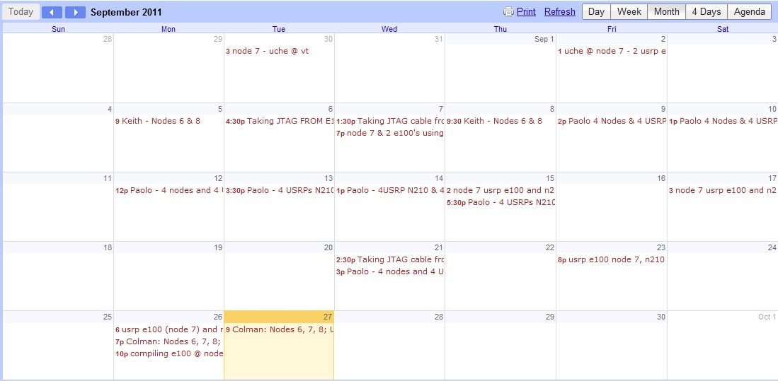
7. All experiments must be scheduled using the Google calendar <ctvr.testbed> specifying all of the following:
· Name of experimenter
· Date and time of booking
· Testbed node number(s)
· Daughtboard(s) of use
· Frequency range(s) of use
8. The testbed should not be used for simulations.
9. The testbed room should be kept secure.
10. Testbed users should sign up to the following mailing lists:
· IRIS support mailing list https://lists.scss.tcd.ie/mailman/listinfo/iris2
· IRIS testbed users mailing list https://lists.scss.tcd.ie/mailman/listinfo/iris-testbed-users for enquiries regarding the Iris testbed.
· IRIS commit mailing list https://lists.scss.tcd.ie/mailman/listinfo/iris2commit for commit notifications.
11. Short descriptions of all experimental work using the testbed should be provided in the projects section of the IRIS wiki https://ntrg020.cs.tcd.ie/irisv2/wiki/ActProjects.
Scheduling an experiment
On receiving testbed login details, the experimenter will also be issued with access to the Google calendar used for scheduling experiments. It is essential to schedule experiments, specifying:
* Which nodes
* Number of USRPs/daughterboards
* Frequencies of operation
* If the spectrum analyser/signal generator is also needed
* Your name
prior to use of the testbed.
An example shot of the calendar is shown below.

| Attachment | Size |
|---|---|
| ctvr_testbed_google_calendar.jpg | 101.79 KB |
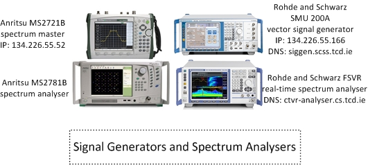
Spectrum analyser remote access
The main spectrum analyser in the testbed room is a Rohde & Schwarz FSVR real-time analyser.
- Host name: ctvr-analyser.cs.tcd.ie
- IP address: 134.226.55.156
- Frequency range: 10Hz - 7GHz
- Frequency range: 10Hz - 7GHz
- Support for IQ analysis (inc. OFDM)
- Maximum sampling rate for IQ acquisition: 128MS/sec
The spectrum analysers are situated as shown in the testbed layout diagram; however, we can easily relocate the receive antenna of the spectrum analyser around the lab if needs be for a certain experiment. We also have in the testbed:
- Rohde & Schwarz SMU 200A - Vector Signal Generator
- Anritsu MS2781B - Signal Analyser
- Anritsu MS2721B - Spectrum Master (handheld spectrum analyser)
Probably the easiest way to acquire data from the Rohde & Schwarz spectrum analyser is using the testbed Windows node "Trinity-8170896" which is accessible via VNC through the ctvr-gateway node. This node runs Rohde & Schwarz IQWizard, a programme which allows simple acquisition of IQ data, in a range of formats. However, remote access directly to the spectrum analyser via VNC is also available.
Remote access via VNC
The spectrum analyser can be accessed from any of the testbed nodes or from the ctvr-gateway server. Information on obtaining access to these nodes can be found here.
* Verify that the analyser is switched on and connected to the network by pinging it using
ping ctvr-analyser.cs.tcd.ie
* Use a VNC client to connect to ctvr-analyser.cs.tcd.ie
Remote control and IQ acquisition using Matlab
It is also possible to perform remote control and IQ acquisition using Matlab.
| Attachment | Size |
|---|---|
| Generators and Analysers - one SigGen.jpg | 87.51 KB |
Test and Trial Ireland
In order to enable research into innovative new technologies, which would require transmission and reception testing within licensed bands, Test and Trial Ireland have the ability to make certain bands in the Irish wireless spectrum available for use. Test and Trial Ireland is a licensing programme which was launched by the Commission for Communications Regulation in Ireland (ComReg).
If the experimenter requires use of licensed bands further details on the programme, as well as information about how to apply for spectrum, are available at http://www.testandtrial.ie/.
![]()
Use of the testbed webcam
In order to view the testbed remotely and to enable experiments with live camera streaming a webcam has been added to the testbed on node05.
The easiest way to veiw the testbed using the webcam is by connecting to node05 via VNC and opening "Cheese Webcam Booth".
We can also reposition the camera if required for certain experiments.
LTE advanced documentation
This section contains basic information about Dresden´s LTE/LTE+ like testbed. Please use the links below to learn more about how the testbed can be used.
If you have any questions do not hesitate to contact us via crew@ifn.et.tu-dresden.de
Introduction
In this section the basic information about the testbed is presented. The possibilities and limitations of the setup are also described.
Basic information
TUD coordinates the test activities that are related with the EASY-C testbed. Cellular use cases and CR-related field trials are provided by the Dresden test bed, which is supervised by TUD.
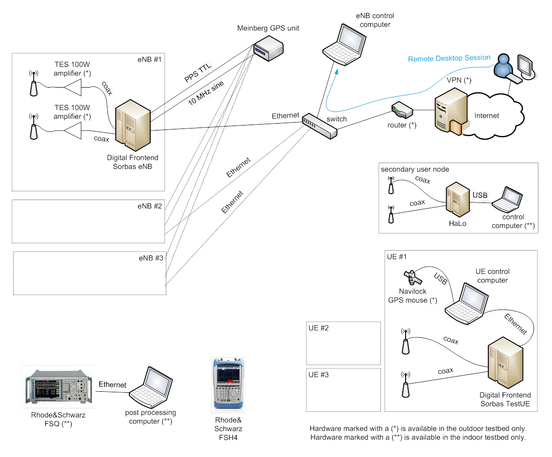
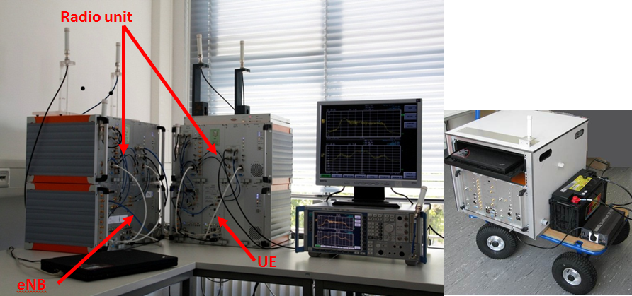
The TUD contribution is based on the EASY-C campus infrastructure, i.e, the EASY-C outdoor lab test bed which is directly operated by the Vodafone Chair research team. An LTE-like cellular infrastructure is used where relevant network parameters are measured such as frame error rates, outage events, throughput or latency. One base station at rooftop level will be used which serves multiple UEs. This BS resides at the faculty of electrical engineering and information technology, TUD. Stationary and mobile user equipment are used. Below are depicted, from left to right: mobile test UE, base station equipment, UE lab equipment.
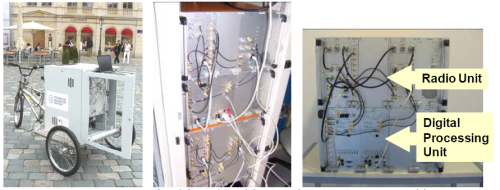
EASY-C test equipment.
External users of the TUD test bed need to install their own equipment at the TUD test site. A predefined test setup is used which provides well defined and reproducible EASY-C LTE traffic – good for the CREW cognitive radio benchmarking initiative. The LTE network parameters are constantly monitored and recorded. The CR transceivers are then activated where the LTE performance parameters are compared for the non-CR and CR case. Hence, it will be possible to benchmark the impact of various CR schemes on a cellular infrastructure through a well-defined set of reproducible test setups.
Another possibility for external users is to connect via Remote Desktop to the TUD indoor test bed to perform experiments with a fixed setup of one eNB, one UE, National Instruments USRP 2920 and one Signalion HaLo device.
Please click on the thumbnail below to get an overview picture of the hardware available in LTE advanced testbed.
| Attachment | Size |
|---|---|
| p01.png | 179.31 KB |
| ltep03.png | 14.91 KB |
Usage of the testbed
Two experimentation setups are available: the indoor lab and the outdoor lab.
In order to conduct experiments in the LTE+ testbed, participants are required to bring their spectrum sensing and/or secondary system hardware to Dresden, if the experiment cannot be performed by a USRP or HaLo device. In order to pre-evaluate certain theories and algorithms, a testbed reference signal in the form of baseband I/Q samples can be provided. Further, during the experiments it is possible to dump transmitted and received signals in the same format. This allows for offline post-processing of the signals, evaluation of the signals and replay in other testbeds.
It is important to distinguish if a downlink (DL) or an uplink (UL) experiment is desired.
In uplink experiments, it is possible to serve up to 4 UEs. The UEs use 1 antenna for transmission, while the eNBs can receive with 1 or 2 antennas. The resolution for scheduling a transmission is 1 ms, which corresponds to 1 TTI (transmission time interval). Scheduling can be done for a total duration of several minutes. The number of occupied PRBs is either 10, 20, 30 or 40 (cf. Table 1). QPSK, 16QAM and 64QAM modulation are supported.
In downlink, up to 4 UEs and up to 4 eNBs can be used simultaneously. The eNBs can transmit with up to 2 antennas and the UEs can receive with up to 2 antennas, thus up to 2 streams per UE can be sent. Time resolution is 1 ms corresponding to 1 TTI (same as UL). The number of occupied PRBs can be 12, 24, 36 or 48 (cf. Table 2).
The evaluation of an experiment happens via dumps of the received signals at the UEs / eNBs. While in the UL, signal dumps can be recorded for all eNBs in synch, the dumping process needs to be initiated manually and out of synch in the DL.
The signal dumps contain the received time samples as well as additional control information. Further processing in Matlab allows derivation of indicators like SINR, BLE, etc. in semi-realtime/offline.
The performance evaluation of experiments can be performed in real-time as well as semi real-time and offline. Real-time measures include
- Received Signal Strength Indicator (RSSI),
- Reference Signal Receive Power (RSRP),
- Path loss, and
- Channel Quality Indicator (CQI; derived from SINR).
In semi real-time, additionally QAM constellations and block error rate (BLER) can be monitored via file dump of I/Q samples and Matlab post processing. Further performance measures could be obtained in offline processing from those file dumps.
Please click on the thumbnail below to get an overview picture of the usage overview in LTE advanced testbed.
Deviations from LTE release 8
As the eNB and UE provide only minimal LTE release 8 (Rel 8) PHY/MAC functionality, it is particularly important to note that the DL frame structure and control channels differ slightly. Differences include:
- PDCCH is always in the second OFDM-symbol (position is variable according to Rel. 8),
- PHICH (HARQ Indicator Channel) is not in the first OFDM symbol and has a different structure/content,
- PCFICH (Control Format Indicator Channel) is not supported, and
- PBCH (Broadcast Channel) is not supported.
Further, the OFDM scheme is used in the uplink. Also, 5 MHz and 10 MHz mode are not supported, thus the testbed operates in 20 MHz mode only.
An overview of the uplink and downlink processing chains can be seen below:
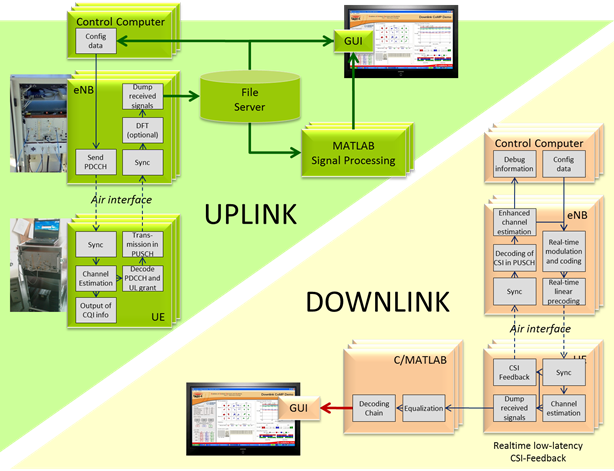
Uplink and Downlink Processing Chain
| Attachment | Size |
|---|---|
| ltep04.png | 164.57 KB |
Getting started with the experiments
If you are new to our testbed, first go through the instructions and see what needs to be done before, during and after the experiment. To get more familiar with the testbed, we recommend you to go through the basic tutorial. After you have understood that, you might want get to know the full possibilities of the testbed, and you can proceed to advanced tutorial.
Instructions for external participants
Before the experiment:
- Contact the testbed staff, make sure the hardware is compatible (frequencies) and the testbed supports all features necessary for the intended experiment
- If necessary for the experiment and after the inital contact with the research staff: Get an account to access the network and computers. Remote desktop access over internet is also possible.
- Make sure there will be enough testbed hardware available (indoor/outdoor?)
- If reasonable, ask for reference signal files to check compatibility with external hardware
- Get familiar using the spectrum analyzer R&S FSQ
- Prepare UE/eNB configuration files or ask testbed staff to do it
During the experiment:
- Carefully check the setup
- Use a terminator when there is no antenna/cable plugged
- Check if all cables are ok
- Make sure you are using the latest version of the config tool to configure the hardware
- Keep a record of the config files you use as you are changing parameters
- Check the signal on the spectrum analyzer, several things can be validated that way
- If in nothing else seems to work reboot and reconfigure the UE/eNB prototype hardware
- When in doubt, ask the testbed staff
After the experiment:
- Put everything back where you took it from
Example experiment
Detection of occupied frequency bands is the foundation for applications of dynamic spectrum access (DSA). In order to convince network operators that DSA is feasible in cellular frequencies, it has to be shown that a reliable detection of their primary signals is possible. In this section, we present an experimental validation of an algorithm and hardware, which can detect the presence of a Long Term Evolution (LTE) signal. In contrast to the classical mono antenna approach, an array of antennas is used, which allows to enhance the detection capabilities, particularly when besides the useful signal there is also interference.
Objectives of experiments
- Reliable sensing in real environment
- Performance gain of multi-antenna vs mono-antenna
- Effectiveness of primary and secondary synchonisation criteria
- Parametrization of sensing algorithm (detection threshhold)
Setup
The multi-antenna LTE sensing platform allows to acquire LTE (I, Q) data and to process them using advanced antenna processing algorithms. As described in the pictures below, the multi-antenna demonstrator is made of:
- A set of 5 antennas,
- A 4-channel receiver,
- A 4-channel acquisition board,
- A GPS system for positioning,
- A laptop for data storage and off-line multi-antenna signal processing.
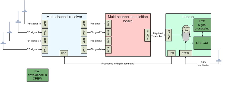
Multi-antenna sensing platform block diagram
Filtering and gain control are applied to the signal in the multi-channel receiver unit, the multichannel acquisition board is used to convert the signals to digital domain and a control computer handles processing and evaluation of the digital samples. The multi-antenna LTE sensing platform is validated with lab tests by measuring sensitivity and co-channel interference rejection with real LTE eNBs. A hardware array simulator consisting of splitters, coupling modules and a set of cables of particular lengths is employed to virtually create a multiantenna, mono-path propagation channel with two directions of arrival.
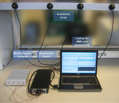
Multi-antenna sensing platform
The main characteristics of the multi-channel receiver are: frequency bands - 1920-1980 MHz / 2110-2170 MHz); bandwidth - 5 MHz; Output intermediate frequency - 19.2 MHz; Noise factor (at maximal gain) <7 dB; Rx gain - 0 to 30dB (1 dB step); Frequency step - 200 kHz; number of Rx channels – 4; Gain dispersion<1 dB; Phase dispersion<6°; Frequency stability <10-7; Selectivity at ±5 MHz >50dB.
The main characteristics of the multi-channel acquisition are: Resolution - 12 bit; internal quartz clock - 15.36 MHz; Number of channels - 4; -3 dB bandwidth >25 MHz; Memory - 8MSamples (i.e. 2MSamples per channel).
Sensitivity tests
For sensitivity measurements, the platform depicted below is used. The level of the BTS is gradually lowered in order to estimate the sensitivity level when using one or four channels for detection processing.
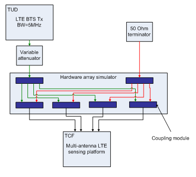
Lab test platform for sensitivity measurements
Interference rejection tests
For interference rejection measurements, the platform described in the picture below is used. The second BTS is considered as the interfering BTS in the following. Its bandwidth was set to 20MHz in order to be able to highly load the OFDM sent symbols. The level of the first BTS is gradually lowered while the level of the second one does not change. The 80% detection limit level is searched when using one or four channels for detection processing.
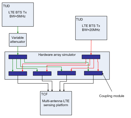
Lab test platform for interference rejection measurements
Results
LTE detection sensitivity level for an 80% detection rate
|
|
1 antenna |
4 antennas |
Multi-antenna gain |
|
Sensitivity level |
-121 dBm |
-129 dBm |
8 dB |
The LTE detection sensitivity performance is summarized in the table above. It is slightly higher to what can be expected (6 dB with 4 antennas). This might be due to a lower sensitivity of the first channel compared to the other three.
LTE rejection capacity for an 80% detection rate
|
|
1 antenna |
4 antennas |
Multi-antenna gain |
|
Sensitivity level of the first BTS |
-92 dBm |
-124 dBm |
32 dB |
|
Rejection capacity of the second BTS |
11 dB |
43 dB |
32 dB |
We can see that, with four antennas, the rejection gain is equal to 32 dB.
For further details refer to: Nicola Michailow, David Depierre and Gerhard Fettweis: “Multi-Antenna Detection for Dynamic Spectrum Access: A Proof of Concept”, QoSMOS Workshop at IEICE 2012
https://mns.ifn.et.tu-dresden.de/Lists/nPublications/Attachments/895/main.pdf
| Attachment | Size |
|---|---|
| ltep12.png | 33.27 KB |
| ltep13.png | 253.64 KB |
| ltep14.png | 14.14 KB |
| ltep15.png | 16.03 KB |
Basic tutorial
This tutorial explains how to set up a basic transmission.
Download this Zip archive with all necessary default configuration files.
Setup the eNB
- Power the hardware
- Sorbas eNB Simulator
- Radio Unit
- eNB control computer
- Configure the eNB
- Open the SimpleProxy 1.3.1 tool
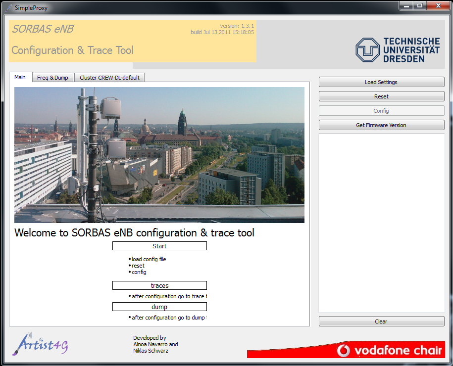
- Click Load Settings and select CREW_DL_config_default_1eNB_2UEs.xml or CREW_UL_config_default_1eNB_2UEs.xml
- Click Reset to reset the eNB
- Wait for eNB broadcast message to appear in the logging box below
- Click Config to send the configuration to the eNB
- Check logging box for errors
- Open the SimpleProxy 1.3.1 tool
Setup the UE
- Power the hardware
- Sorbas Test UE
- Radio Unit
- UE control computer
- Configure the UE
- Open the TestUE Config tool
- Select the System Config tab
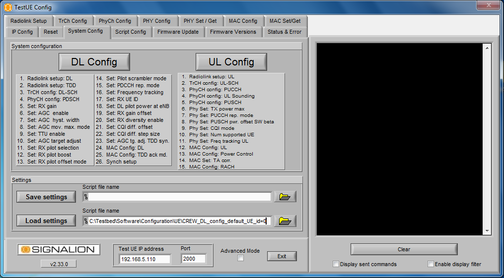
- Click Load settings and select CREW_DL_config_default_UE_id=0 or CREW_UL_config_default_UE_id=0
- Click DL config and wait for UE response
- Click UL config and wait for UE response
- Trace
- Open the TestUE Trace tool
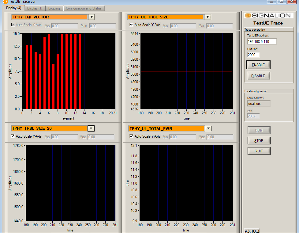
- Select the Display (4) tab
- Click Enable
- Click Run
- Open the TestUE Trace tool
The system is now running. Check spectrum on R&S FSQ. 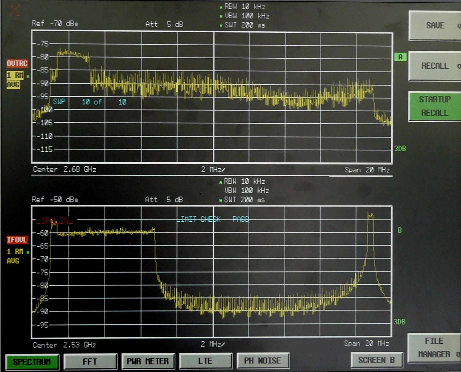
Record IQ data dumps
- Dump at the eNB
- Open the SimpleProxy 1.3.1 tool
- Click Freq && Dump tab
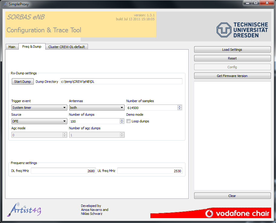
- Click Start Dump
- Dump at the UE
- Browse into the directory of the UE_dump_tool
- Click start.bat
- Process IQ dumps
- Extract IQ samples and AGC values with dumpDemux.m script
- Perform further processing in Matlab
Advanced tutorial
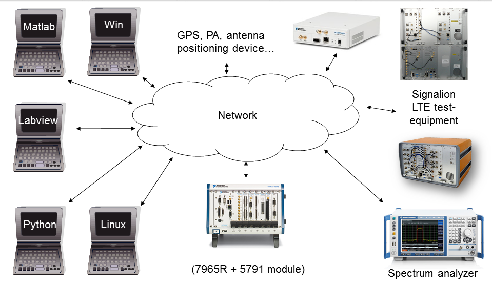
Besides the manual, gui-based control for test bed related programs and devices, script controlled measurements are also possible. This approach developed at the Vodafone chair is called TestMan. The basic idea is to provide a common interface to exchange data, commands and status messages between different application, running on the same or distributed systems and written in different languages.
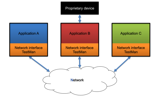
TestMan is based on the Microsofts .NET framework, which similar to java, is platform independent. So even a Linux computer can make use of .NET programs if the Mono project is used. In three important languages Matlab, Labview and Python it is possible to use dynamic link libraries (DLL). Therefore TestMan is a DLL which can be loaded into the specific application or script and it makes sure that data is transferred over the network from one Application to another, respectively to a group of applications.
TestMan uses two different network techniques to exchange information’s: For SNMP like status messages and commands UDP multicast is used whereas TCP peer to peer connection comes into place for transferring bigger data.
To distinguish between different applications a type and an ID are introduced for every application. So it is possible to group similar applications together and the TestMan DLL filters out messages which are intended for other applications.
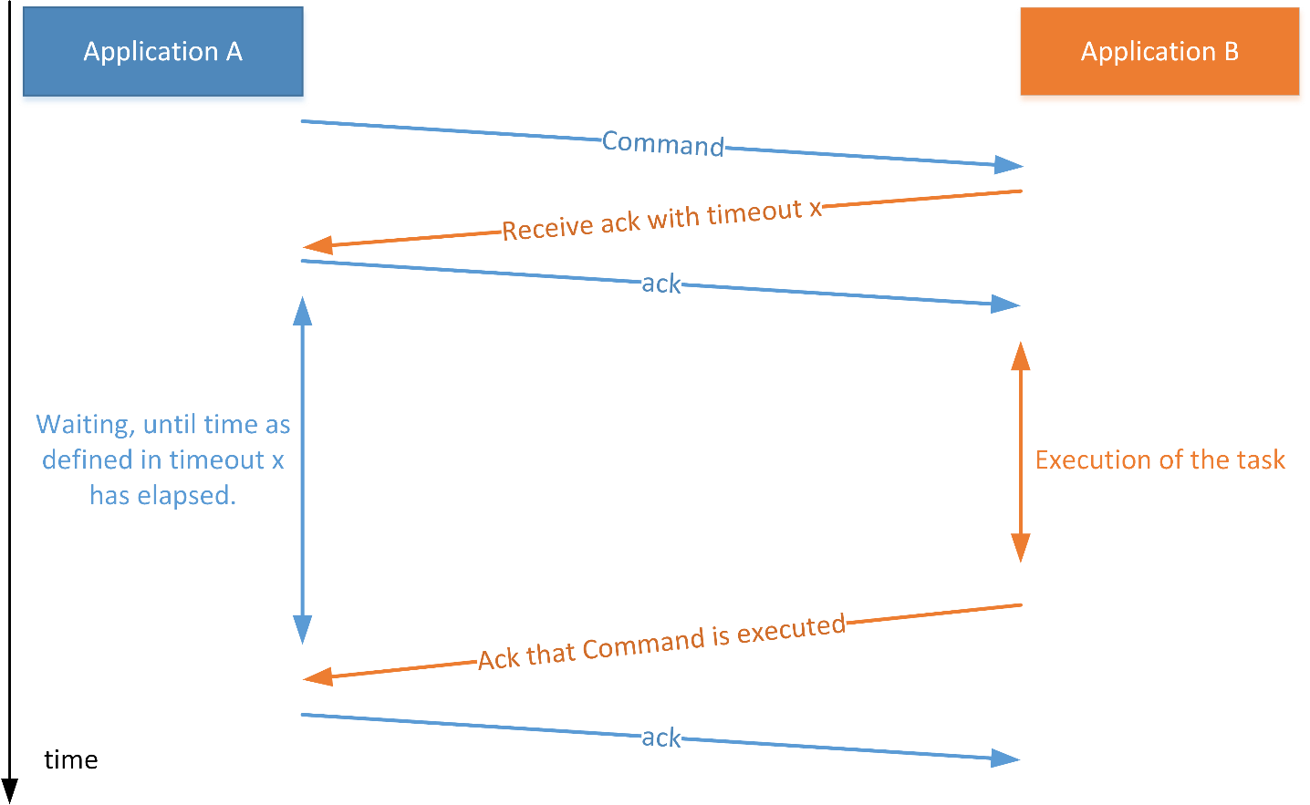
UDP packets can be thrown away by network elements like routers and switches. For a status messages this is not always a problem, but definitely when a command is send. To mitigate this problem TestMan uses 4-way handshaking for commands as stated in the following figure.
The following picture shows an example how an OFDM-Transmitter can be implemented using TestMan.
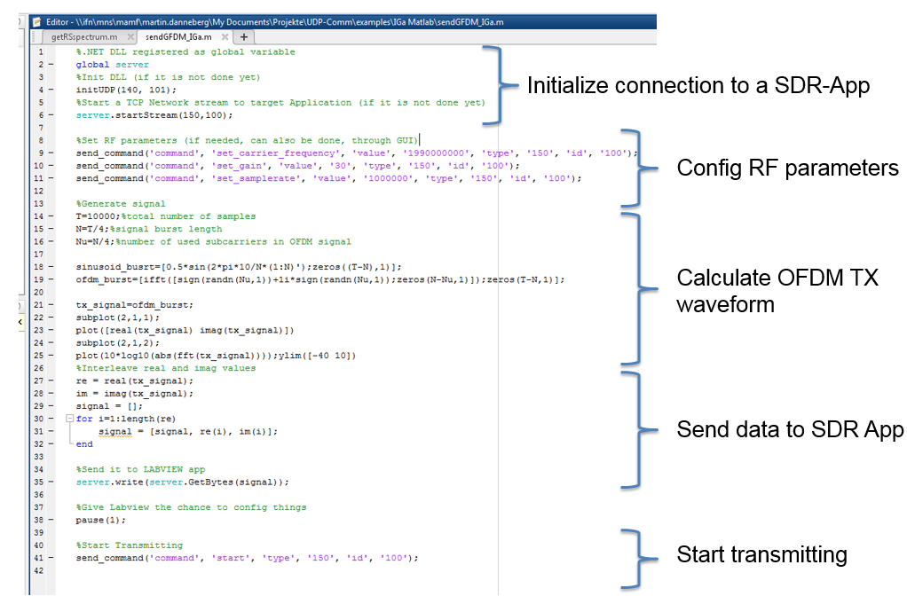
Are more detailed example code will be published soon.
| Attachment | Size |
|---|---|
| TestMan_Commands.png | 83.12 KB |
| matlab-example.png | 180.36 KB |
| TestMan_Devices.png | 243.01 KB |
| TestMan_Overview.png | 41.9 KB |
Hardware
In this section you can find detailed description of the hardware used in the testbed.
Configuration
Dresden’s LTE/LTE+ like testbed was set up in 2008 as part of the Easy-C project (www.easy-c.com).
The signal processing hardware includes:
- Sorbas602 eNodeB Simulators with ZF Interface to a Sorbas Radio Unit ("ZF Interconnect”)
- Sorbas202 Test UEs with ZF Interface to a Sorbas Radio Unit ("ZF Interconnect”)
- Sorbas472 Radio Units, by Signalion: EUTRAN band VII (2.5 - 2.57 GHz and 2.62 - 2.69 GHz) as well as close to band I (1.98-2 GHz and 2.17-2.19 GHz), 20MHz bandwidth, Tx power approx. 15dBm (indoor) and approx. 30dBm (outdoor), supports up to two Tx and two Rx channels.
They were supplied by Signalion (www.signalion.com). The eNBs and UEs are connected through IF interconnects at 70MHz with the radio unit frontend. The hardware supports up to two Tx and two Rx channels for MIMO capability. The testbed operates in EUTRAN band VII (DL @ 2670-2690 MHz / UL @ 2550-2570 MHz) with fixed bandwidth of 20MHz and in FDD mode.
The LTE testbed at TUD has been upgraded with a new spectrum license in the 2.1 GHz band (1980 MHz to 2000 MHz and 2170 MHz to 2190 MHz). This step was necessary to ensure the continuous operation of the LTE testbed when the spectrum license for 2.6 GHz is withdrawn due to commercial use of the corresponding frequencies in Germany. Along with the license, several nodes have been equipped with 2.1 GHz frontends. Note that only the RF parts have been replaced, while LTE eNB and UE baseband processing remains unaffected due to the modular structure of the equipment. Further note that as long as the 2.6 GHz license is not withdrawn, those frequencies are still available for experimentation.
The operation of the new equipment has been successfully tested. The internal US5 experiment “LTE Multi-Antenna Sensing” has been conducted in the 2.1 GHz frequency range.
Base station (eNB) and mobile terminal (UE) nodes each are connected to a host PC and configured with text files in XML format. The host computer also manages measurements of the received signals and stores them in dumps. At the eNBs, a GPS unit is used for synchronization, while the UEs employ GPS for position tracking. Additionally, UEs can be powered by a mobile power supply if necessary.
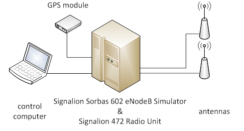
Configuration of a baste station node (eNB)
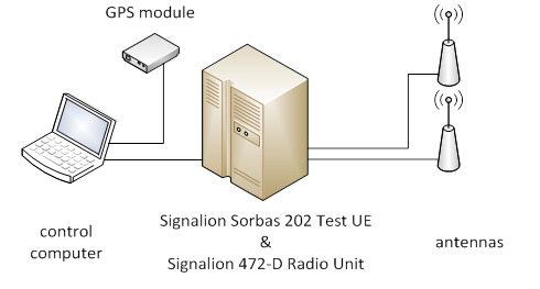
Configuration of a mobile terminal node (UE)
All UEs in the testbed, as well as the indoor eNBs are equipped with Kathrein 800 10431 omnidirectional antennas. The antennas of the outdoor eNBs are sectorized and of type Kathrein 800 10551. You can find detailed information about these antennas here:
http://www.kathrein-scala.com/catalog/80010431.pdf
http://www.kathrein.de/en/mcs/catalogues/download/99811214.pdf
Other testbed equipment includes six batteries that can power an individual UE for around 2-4 hours, GPS receivers for time synchronization, various cables, attenuators and splitters. Measurement equipment includes spectrum analyzers Rohde & Schwarz FSH4, Rohde & Schwarz FSQ8 and Rohde & Schwarz TSMW. For more details click on following links:
R&S FSH4 data sheet:
http://www.test-italy.com/occasioni/2013/rs_fsh8-18/FSH_dat-sw_en.pdf
R&S FSQ8 data sheet:
R&S TSMW operating manual:
http://www.rohde-schwarz.de/file_9446/TSMW_Operating_Manual.pdf
R&S TSMW software manual:
http://www.rohde-schwarz.de/file_11255/TSMW_Interface_and_Programming_Manual.pdf
| Attachment | Size |
|---|---|
| ltep05.png | 29.64 KB |
| ltep06.png | 28.13 KB |
Indoor and outdoor setups
For the CREW project, two experimentation setups are available.
The indoor lab features 5 eNBs and 4 UEs. While the hardware itself is stationary, the Tx and Rx antennas can be positioned anywhere in the lab room. Further, four additional UEs are mounted on studio racks/carts and can be moved within the building. The approximate transmit power is 15 dBm.
The outdoor lab consists of two base station sectors that are fixed on two opposing corners of the faculty building, approximately 150 m apart. In addition to the mobile indoor UEs from setup 1, three rickshaw UEs are available for outdoor experiments in the vicinity of the building. There are also 6 batteries which can supply an UE for around 2-4 hours. The transmit power is approximately 30 dBm.
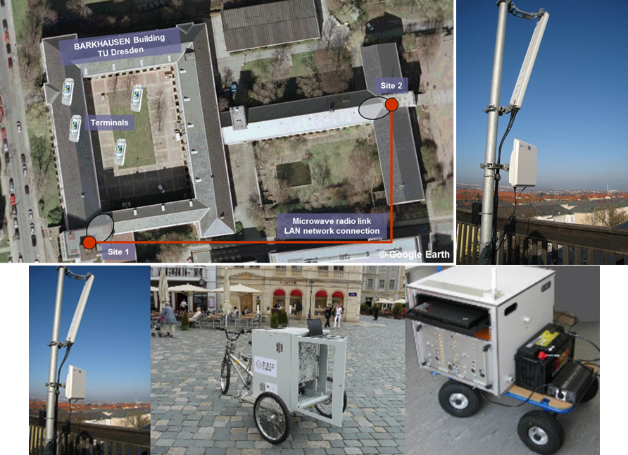
Outdoor setup
Indoor setup
| Attachment | Size |
|---|---|
| ltep07.png | 918.06 KB |
| ltep08.png | 494.97 KB |
Secondary System
The Signalion Hardware-in-the-Loop (HaLo) is a platform designated to simplifying the transition from simulation to implementation. To support cognitive radio setups that consider a primary/secondary user configuration, the LTE testbed has been extended by a HaLo node that can take the role of the secondary user. On the HaLo device, a novel modulation scheme called Generalized Frequency Division Multiplexing (GFDM) is now available.
This enables experimenters to consider experiment setups in LTE testbed, where the LTE system can act as a monitored primary system, while the GFDM system can run as an interfering secondary system.
HaLo Concept
The HaLo consists of a wireless transceiver that can operate in the 2.6 GHz frequency band. The concept is such, that complex valued data samples are transmitted to the device’s memory via USB from a control computer. The samples can be either read from a previously recorded file or generated on the fly e.g. by a Matlab script. The signal is transmitted over the air and received in a similar way. The device digitizes the signal and stores complex valued samples to an internal memory before they are fed back via USB to the control computer.
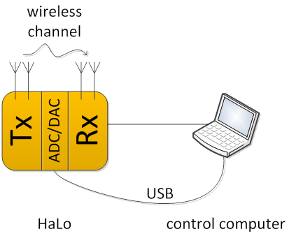
The HaLo setup
Note that due to limitations in the HaLo’s internal memory real-time operation is not possible.
GFDM Theory
The transmission scheme chosen to be implemented on the HaLo device to act as a secondary system in the testbed is a novel, non-orthogonal and flexible modulation scheme called GFDM. The concept is such that a multicarrier signal is transmitted, quite similar to the well know and established OFDM scheme, however one of the differences is in the pulse shaping of the individual subcarriers. This step allows shaping of transmissions and produces a signal with particularly low out-of-band radiation, which is a very desirable property in cognitive radio. For further details please refer to:
https://mns.ifn.et.tu-dresden.de/Lists/nPublications/Attachments/826/Michailov_N_VTCfall12.pdf
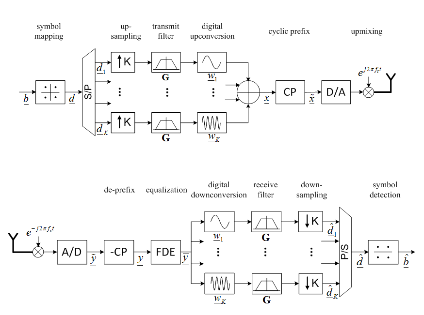
GFDM transmitter and receiver block diagram
| Attachment | Size |
|---|---|
| ltep09.png | 26.04 KB |
| ltep10.png | 51.37 KB |
Tools
SimpleProxy 1.3.1
This tool is installed on all eNB control computers and is used to connect to an eNB, load a configuration and dump IQ data at eNB.
TestUE Config
This tool is installed on all UE control computers and is used to configure an UE.
Test UE Trace
This tool is installed on all UE control computers and is used to monitor UE activity in real-time
UE_dump_tool
This tool is installed on all UE control computers and is used to record the UE's IQ data dumps.
GFDM chain
This tool is used to generate a secondary user signal and control the HaLo node.
FAQ
TWIST documentation
Browse the sections below for information about the TWIST testbed.
!!! THIS INFORMATION MIGHT BE OUTDATED !!!
Updated documentation can be found at https://www.twist.tu-berlin.de/
Introduction and overview of capabilities
TKN Wireless Indoor Sensor network Testbed (TWIST)
The TKN Wireless Indoor Sensor network Testbed (TWIST), developed by the Telecommunication Networks Group (TKN) at the Technische Universität Berlin, is a scalable and flexible testbed architecture for experimenting with wireless sensor network applications in an indoor setting. The TWIST instance deployed at the TKN group includes 204 sensor nodes and spans three floors of the FT building on the TU Berlin campus, resulting in more than 1500 square meters of instrumented office space. TWIST can be used locally or remotely via a webinterface.
Additonal components
In addition to TWIST, which is a fixed testbed infrastructure, CREW experiments involving mobility can be carried out in the TKN premises using additional equipment. The use of this equipment requires additional support at the TKN premises. This can be achieved either by experimenters beeing present at the premisises or by additional support from TWIST staff.
The additional components are:
- 2 mobile robots: Turtlebot-II based on Kobuki mobile base and a Microsoft Kinect 3D sensor. The robot runs ROS (an open-source, meta-operating system) and it can be programmed to follow certain trajectories in the TWIST building. Shimmer2 sensor nodes or WiSpy devices (see below) can be mounted on the robot, e.g. to record RF environmental maps, or perform experiments emulating body area networks (BANs) as well as experiments involving interaction between a mobile network and the fixed TWIST infrastructure.
- 8 Shimmer2 nodes, which are wearable sensor nodes similar to the popular TelsoB platform and can be attached to a person (or robot).
- 10 WiSpy 2.4x USB Spectrum Analyzers, which are low-cost devices to scan RF noise in the 2.4 GHz ISM band.
-
3 ALIX2D2 embedded PCs equipped with Broadcom WL5011S 802.11b/g cards.
Getting started: tutorials
Below you find information on how to get started using the TWIST testbed. Most steps involve remote access via the TWIST web interface, but there is also a more advanced tutorial on how to control TWIST via the cURL command line tool.
Requesting a user account
To access the TKN instance of the TWIST web interface you need to have registered an account. If you are not yet registered, go to the TWIST web interface where you should see the following welcome page:
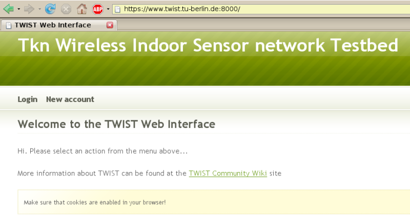 Make sure that your browser has cookies enabled and click on "New account". In the form fill in your name, email address and choose a username (at least 6 characters) and a password. Make sure you confirm the password and answer the spam control question. Then press the "Request" button; if you filled in the form correctly you will see a new page saying "Successful account request". Now go to the TWIST terms of use page. Copy and paste the content of this page into an email, add the requested information (the nature of the intended experiments, etc.) and send this email to the TWIST administrator (email address is given on the same webpage). Please also make sure that you explain your relationship to the CREW project. The last step in obtaining an account is in the responsibility of the administrator, and you will be notified by email when your account has been activated. If there are any problems, please contact Mikolaj Chwalisz.
| Attachment | Size |
|---|---|
| TWIST_login_screen.png | 96.54 KB |
Running a simple experiment
Installing a node image
In this section we install the TinyOS 2 Oscilloscope application on a set of Tmote Sky nodes in the TKN TWIST testbed. The Oscilloscope application is described in the TinyOS 2 tutorial 5. After you have compiled the application with make telosb open a web browser and access the TWIST web interface. Press the "Login" button, enter your username and password and then click on "Sign in". If you have not yet registered a TWIST user account take a look at this tutorial page.
You will see a welcome page where you have three options: manage and update your account settings ("My Info"), schedule and control jobs in the testbed ("Jobs") or logout ("Logout"). Click on "Jobs" and you will see a list of scheduled jobs, i.e. the currently active jobs as well as pending future jobs. Take a close look at the list and find a time period for which Tmote/TelosB nodes are not reserved by someone else. Then click on "Add" and you will see the Job Management page as follows:
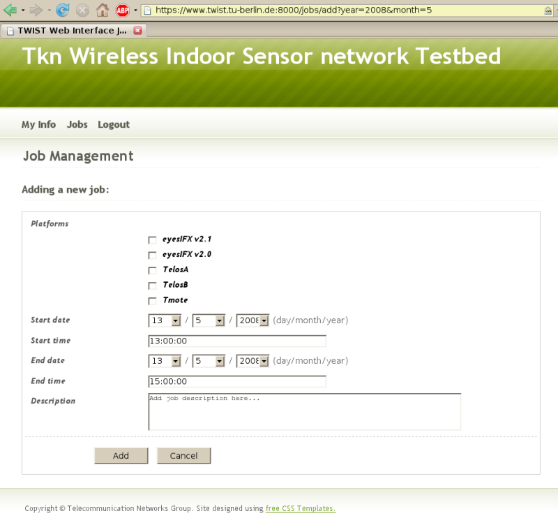
Under "Platforms" select Tmote; then choose a "Start/End date" and "Start/End time" such that the time interval is not overlapping with other jobs, which you checked in the previous step. You cannot make a real mistake here, because the system will automatically check for and not permit jobs that are overlapping in time if they use the same mote platform. However, different platforms (eyesIFX vs. Tmote) may be used concurrently. In the field "Description" enter a short note on what you plan to do in your job, such as "Testing the T2 Oscilloscope application", then click on "Add". If the time interval that you entered was accepted you will be taken back to the list of scheduled jobs, otherwise you get an error message and need to adapt the values.
The list of "Scheduled jobs" should now include your job. Your entry is likely to have gray background colour, meaning that it is registered but not yet active. The current system time is always shown in the upper right corner of the page and once your job becomes active -- its start time is shown in the column "Start" -- the background colour of your entry will turn yellow (you need to click the reload button of your browser).
When your job is active apply a tick mark at the left side of the entry and press the "Control" button at the bottom (the "Edit" button would be used to change the time of your job and with the "Delete" button you can remove your job).
Hint: When your job is active (during a experiment) you can still extend its "End time" by clicking on "Edit" on the "Jobs" page, provided that the new "End time" does not overlap with other registered jobs.
After you have clicked the "Control" button you will see the page for controlling your active job as shown in this figure:
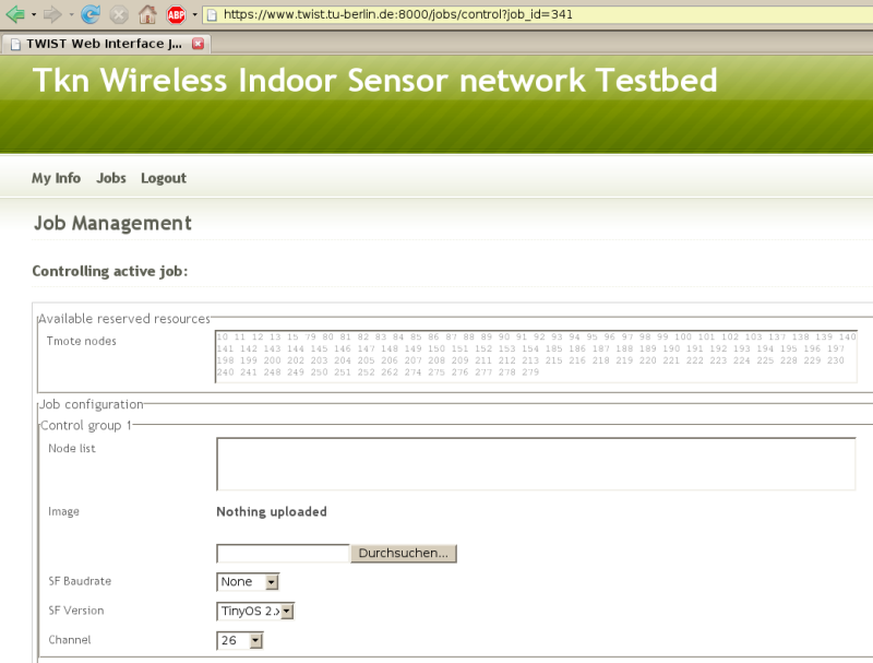
This page is divided into the list of Tmote node IDs available in the testbed ("Available reserved resources"), a section for submitting up to three different program images to be programmed on a subset of the nodes ("Job configuration") and a set of buttons (on the bottom, not shown in Figure 3) to perform some actions, such as installing the image(s) on the nodes.
For the TinyOS 2 Oscilloscope application we want to install the Oscilloscope program image on some Tmote nodes, and one node will need to act as gateway and will be programmed with the TinyOS 2 BaseStation application (see TinyOS 2 tutorial 5). Because we will install two different application images, in the "Job configuration" field we will use two of the three "Control group" sections: the "Control group 1" section for the Oscilloscope application and the "Control group 2" section for the BaseStation application.
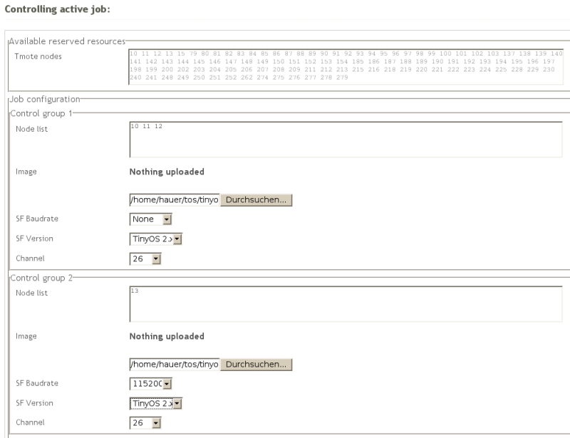
In the "Control group 1" section, enter in the "Node list" field a whitespace-separated list of the node IDs on which the the Oscilloscope is to be programmed, let's say 10 11 12. For convenience you can copy & paste from the list of IDs shown on top in the "Available reserved resources" list.
Then click on the "browse..." button next to the "Image" field just below the "Node list" field. Select the Oscilloscope image, which is the main.exe in your local tinyos-2.x/apps/Oscilloscope/build/telosb (you must have compiled the Oscillocope application with "make telosb" before). The "SF Baudrate" and "SF Version" fields control whether a SerialForwarder will be started for all nodes in the respective "Node list". Since we only need a SerialForwarder for the BaseStation application, we don't change the values (leaving it "None", "TinyOS 2.x"). Finally, "Channel" is the IEEE 802.15.4 channel to be used by the Tmote Sky radio CC2420 (if you change the channel for the Oscilloscope application, make sure that you do the same for the BaseStation application). In fact, the value of the CC2420_DEF_CHANNEL symbol inside your progam image will be replaced by the value of the "channel" field and thus, if your application includes the TinyOS 2 CC2420 radio stack, you can still modify the default radio channel after you have compiled the image.
Hint: The node ID is another symbol that is modified for each node individually before programming the image. It is accessible via TOS_NODE_ID in a TinyOS application.
We use the "Control group 2" section for installing the BaseStation program image on another node. In the "Node list" field enter 13 (or whichever node ID you want to use for the BaseStation application) and under "Image" click "browse..." and select the main.exe from your local tinyos-2.x/apps/BaseStation/build/telosb folder (you must have compiled the BaseStation application with "make telosb" before). Because we want to later establish a serial connection to the BaseStation node, select the pull-down menu under the "SF Baudrate" field and choose a serial baudrate. Whenever this field has a value other than None a SerialForwarder will be started for all nodes in the respective "Node list". The default baud rate for the "TelosA", ",TelosB" and "Tmote" platforms is 115200 baud.
Hint: You can change the baud rate for a telos node by modifying tinyos-2.x/tos/platforms/telosa/TelosSerialP.nc (this file is included by telosa, telosb and tmote platform). Make sure you recompile your application after changing the file.
The "SF Version" field defines the version of the Serial Forwarder protocol. Because we are using a TinyOS 2 applications select "2" (for a TinyOS 1 application you would select "1"). If the "SF Baudrate" field is None then the "SF Version" is ignored. Finally, make sure you select the same "Channel" as the one for the Oscilloscope application. Your configuration should now look like the one shown the next figure:
To actually program the images on the nodes scroll down, press the "Install" button and wait. After not much longer than 1 minute you should see a page with the "Execution log". Check for possible errors (any line "Could not find symbol [...] ignoring symbol" is only telling you that the respective symbol was not found/changed in the application image) and scroll down to the bottom where you can find a summary of the "Install" operation. Here you can also see that a SerialForwarder has been started for node 13:
To forward SF e.g. for node 13 use: ssh -nNxTL 9013:localhost:9013 twistextern@www.twist.tu-berlin.de
In the next section we will establish an ssh tunnel to the TWIST server and connect to the SerialForwarder of the BaseStation node. The remainder of this section summarizes the fields and options for controlling an active job over the web interface.
The following table describes the fields in the "Job configuration" section:
Field Meaning Node list Whitespace separated list of node IDs on which the image will be programmed Image The image to be programmed on the nodes in the "Node list" SF Baudrate Whether a SerialForwarder is started for each of the nodes in "Node list"
and what baudrate it will useSF version The version of the SerialForwarder: use 1 for TinyOS 1.x and 2 for TinyOS 2.x Channel The CC2420 radio channel
The following table describes the buttons on the bottom of the "Controlling active job" page:
Button Meaning Install Installs the image(s) on the node(s) specified in the above "Job Configuration"
section; SerialForwarders will be started (if selected) and nodes are powered onErase Programs the TinyOS Null application on the selected set of nodes Reset Resets (powers off & on) the selected set of nodes Power On Cuts the USB power supply for the selected nodes Power Off Enables the USB power supply for the selected nodes Start SF Starts a SerialForwarder for the selected nodes Stop SF Stops the SerialForwarder for the selected nodes Start Tracing Stores the serial data output from the nodes in a trace file Stop Tracing Stops storing data in a trace file
By pressing the "Start Tracing" button the serial data output from all nodes are automatically stored to a trace file. This file can be accessed via the job control page by pressing the "Traces" button (with your job checked). If you want to use automatic tracing then it is recommended that during install you select the correct "SF Baudrate" and "SF Version". After the install process, you can then simply click on "Start Tracing" without having to manually start the serial forwards.
Exchanging Data via the Serial Connection
Through the previously described "Install" operation a SerialForwarder for the BaseStation node was started. In order for your tinyos-2.x/apps/Oscilloscope/java/Oscilloscope.java client to connect to this SerialForwarder, you first need to establish an SSH Tunnel to forward the port of the SerialForwarder to your machine. At the very end of the execution log you find the syntax for this SSH command (type it into a shell):
ssh -nNxTL 9013:localhost:9013 twistextern@www.twist.tu-berlin.de
Once you have forwarded the port you can access the remote SerialForwarder like a local one. However, when you start your client application make sure that it attaches to the correct port as specified in the SSH Tunnel (the above command forwards the remote port to your local port 9013). For example, to start the JAVA Oscilloscope client you would first need to set the MOTECOM environment variable as follows:
export MOTECOM=sf@localhost:9013
Now you can start the Oscilloscope GUI by typing:
.\run
in the tinyos-2.x/apps/Oscilloscope/java directory as described in TinyOS 2 tutorial 5.
You should now see an Oscilloscope GUI like the one described in the TinyOS tutorial.
| Attachment | Size |
|---|---|
| TWIST_job_management.png | 104.83 KB |
| TWIST_active_job_control.png | 89.52 KB |
| TWIST_example_job_control.png | 61.46 KB |
Using cURL for automated control
cURL is a command line tool that can, among other things, transfer files and POST web forms via HTTPS. It can thus be used to automate sequences of operations on the testbed, such as installing an image or powering a node off. Before you can actually control your job you need to authenticate via cURL (Step 1) and find you job ID (Step 2). Afterwards you can control your job (Step 3) and download traces (Step 4) associated with your job ID. The following steps list the relevant cURL commands.
Step 1: Authenticate
Use the following format to authenticate and store the secure cookie for the future requests (replace YOUR_USER_NAME and YOUR_PASSWORD with your username and password, respectively):
curl -L -k --cookie /tmp/cookies.txt --cookie-jar /tmp/cookies.txt -d 'username=YOUR_USER_NAME' -d 'password=YOUR_PASSWORD' -d 'commit=Sign in' https://www.twist.tu-berlin.de:8000/__login__
Note that all data fields have to be URL encoded either implicitly using --data-urlencode or explicitly (in case you have special characters in username/password)
Step 2: Find the job_id
You need to know the job_id before you can use curl to control it. This can also be done by fetching and parsing the jobs page with cURL, maybe passing the output through "tidy"
curl -L -k --cookie /tmp/cookies.txt --cookie-jar /tmp/cookies.txt https://www.twist.tu-berlin.de:8000/jobs | tidy
Step 3: Control
The following is a list of examples on how to control a job. Make sure that you replace the job_id and node IDs.
-
Erase - For job_id 346, erase nodes 12 and 13:
curl -k --cookie /tmp/cookies.txt --cookie-jar /tmp/cookies.txt -F __nevow_form__=controlJob -F job_id=346 -F ctrl.grp1.nodes="12 13" -F erase=Erase https://www.twist.tu-berlin.de:8000/jobs/control
-
Install - For job_id 346, install TestSerialBandwidth on nodes 12 and 13 and start serial forwarders:
curl -k --cookie /tmp/cookies.txt --cookie-jar /tmp/cookies.txt -F __nevow_form__=controlJob -F job_id=346 -F ctrl.grp1.nodes="12 13" -F ctrl.grp1.image=@/home/hanjo/tos/tinyos-2.x/apps/tests/TestSerialBandwidth/build/telosb/main.exe -F ctrl.grp1.sfversion=2 -F ctrl.grp1.sfspeed=115200 -F install=Install https://www.twist.tu-berlin.de:8000/jobs/control
-
Power Off - For job_id 346, power off nodes 12 and 13:
curl -k --cookie /tmp/cookies.txt --cookie-jar /tmp/cookies.txt -F __nevow_form__=controlJob -F job_id=346 -F ctrl.grp1.nodes="12 13" -F 'power_off=Power Off' https://www.twist.tu-berlin.de:8000/jobs/control
-
Power On - For job_id 346, power on nodes 12 and 13:
curl -k --cookie /tmp/cookies.txt --cookie-jar /tmp/cookies.txt -F __nevow_form__=controlJob -F job_id=346 -F ctrl.grp1.nodes="12 13" -F 'power_on=Power On' https://www.twist.tu-berlin.de:8000/jobs/control
-
Start Tracing - For job_id 346, start tracing on nodes 12 and 13:
curl -k --cookie /tmp/cookies.txt --cookie-jar /tmp/cookies.txt -F __nevow_form__=controlJob -F job_id=346 -F ctrl.grp1.nodes="12 13" -F 'start_tracing=Start Tracing' https://www.twist.tu-berlin.de:8000/jobs/control
-
Stop Tracing - For job_id 346, stop tracing on nodes 12 and 13:
curl -k --cookie /tmp/cookies.txt --cookie-jar /tmp/cookies.txt -F __nevow_form__=controlJob -F job_id=346 -F ctrl.grp1.nodes="12 13" -F 'stop_tracing=Stop Tracing' https://www.twist.tu-berlin.de:8000/jobs/control
Step 4: Collect data
To collect the specific trace file from archived job 336
curl -g -k --cookie /tmp/cookies.txt --cookie-jar /tmp/cookies.txt -d 'job_id=339' -d 'trace_name=trace_20080507_114824.0.txt.gz' -o trace_20080507_114824.0.txt.gz https://www.twist.tu-berlin.de:8000/jobs/archive/traces/download
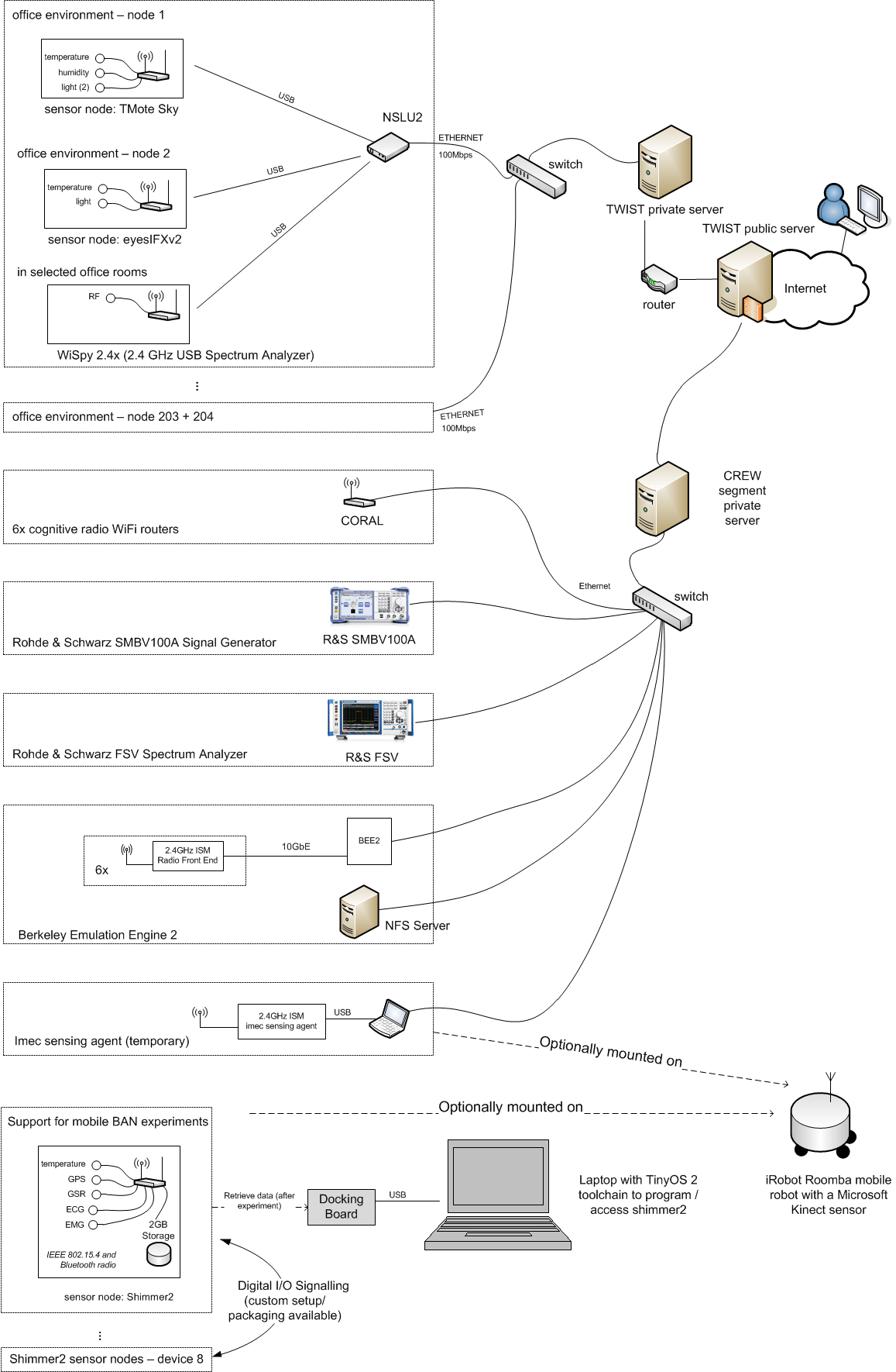
Hardware and testbed lay-out
The TKN Wireless Indoor Sensor network Testbed (TWIST), developed by the Telecommunication Networks Group (TKN) at the Technische Universität Berlin, is a scalable and flexible testbed architecture for experimenting with wireless sensor network applications in an indoor setting. It provides basic services like node configuration, network-wide programming, out-of-band extraction of debug data and gathering of application data, as well as several novel features:
- experiments with heterogeneous node platforms
- support for flat and hierarchical setups
- active power supply control of the nodes
The self-configuration capability, the use of hardware with standardized interfaces and open-source software makes the TWIST architecture scalable, affordable, and easily replicable. The TWIST architecture was published in this paper.
The TWIST instance deployed at the TKN group is one of the largest academic testbeds for indoor deployment scenarios. It spans the three floors of the FT building at the TU Berlin campus, resulting in more than 1500 square meters of instrumented office space. Currently the setup is populated with two sensor node platforms:
- 102 TmoteSky nodes, which are specified in detail here.
- 102 eyesIFXv2 nodes; this platform is an outcome of the EU IST EYES project. The platform is based on an MSP430 MCU and the TDA5250 transceiver, which operates in the 868 MHz ISM band using ASK/FSK modulation with data-rates up to 64 Kbps. A summary of the platform's hardware components is given, for example, in this paper.
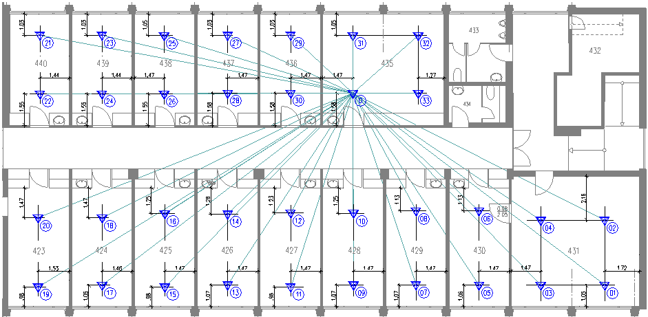
In the small rooms, two nodes of each platform are deployed, while the larger ones have four nodes. The setup results in a fairly regular grid deployment pattern with intra node distance of 3m. The following shows the node placement on the 4th floor of the building (floors 3 and 2 have a very similar layout):
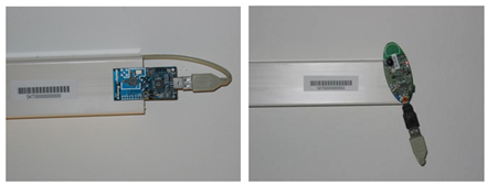
The testbed architecture can be divided into three tiers. The sensor nodes form the lowest tier, they are attached to the ceiling as visualized in the following figure, which shows a Tmote Sky and an eyesIFXv2 node in one of the office rooms:
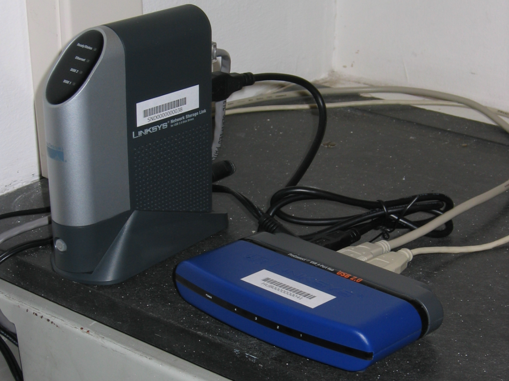
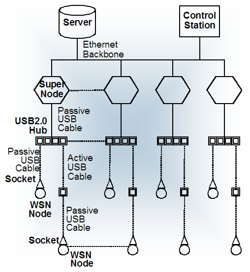
Sensor nodes are connected via USB cabling and USB hubs to the testbed infrastructure. If TWIST only relied on the USB infrastructure, it would have been limited to 127 USB devices (both hubs and sensor nodes) with a maximum distance of 30 m between the control station and the sensor nodes (achieved by daisy-chaining of up to 5 USB hubs). Therefore the TWIST architecture includes a second tier: so-called "super nodes" which are able to interface with the previously described USB infrastructure. We are using the Linksys Network Storage Link for USB2.0 (NSLU2) device as super nodes as depicted in the following picture:
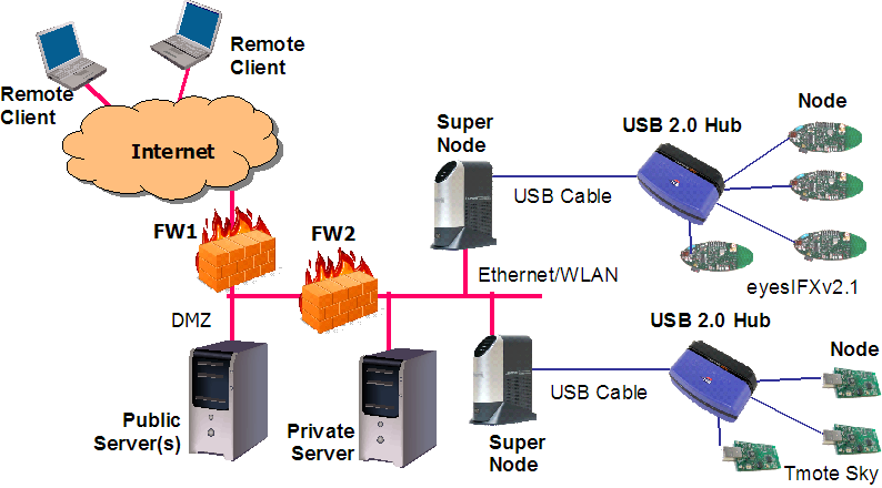
The third and last tier of the architecture is the server and the control stations which interact with the super nodes using the testbed backbone. The server, among other things, implements a PostgreSQL database that stores a number of tables including configuration data like the registered nodes. It also provides remote access via a webinterface. The following figure provides a general overview of the TWIST hardware architecture:
The hardware instantiation of the TWIST hardware architecture at the TKN group is shown in this figure:
| Attachment | Size |
|---|---|
| TWIST_components.png | 115.05 KB |
| TWIST_architecture.png | 70.2 KB |
| TWIST_slug.png | 1.04 MB |
| TWIST_telos.png | 1.01 MB |
| TWIST_floorplan.png | 25.42 KB |
| TWIST_tmote_and_eyesIFXv2.png | 66.14 KB |
System health monitoring
The system health of the TKN TWIST instance is constantly monitored using the CACTI monitoring tools:
You can either use the CACTI System Health Summary, which displays information on the utilization of the testbed server and super node status. The information is updated every 30 min.
Or you can access the CACTI System Health Browser to see more fine-grained information on some particular systems components (please use account name "guest" and password "guest" to get access to the public data.)
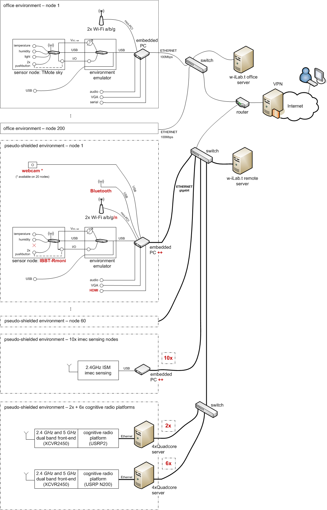
w-iLab.t documentation
All documentation for the w-iLab.t Office and Zwijnaarde is now available here.
IMEC sensing engine documentation
To achieve dynamic spectrum access, sensing techniques are crucial. The IMEC Sensing Engine can add sensing capabilities to radio systems and enable the evaluation of cognitive network solutions. Both hardware and firmware are reconfigurable, allowing to support and evaluate a wide range of sensing applications. A CREW application programming interface (API) is implemented as a Linux library, to ease the writing of new applications in a standard way. Currently, eight prototypes are deployed in the CREW w-iLab.t test-bed. These are connected by means of an USB interface to their corresponding Zotac nodes. Figure 1 shows an unpackaged version of the IMEC sensing engine with scaldio frontend.
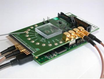
Figure 1. Unpackaged IMEC sensing engine with a Scaldio-2B wide band front-end.
At present seven units are deployed in the w-iLab.t Zwijnaarde testbed and one is deployed in the w-iLab.t office testbed. An introduction of how to access the IMEC sensing nodes in the CREW w-iLab.t facility is available on following pages:
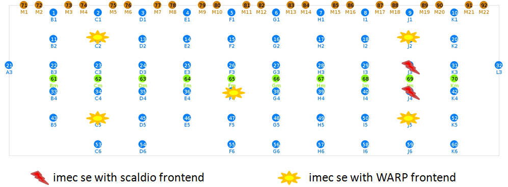
Figure 2. Deployment of IMEC sensing engine in the CREW Zwijnaarde w-iLab-t test-bed
The next sections focus on developing firmware for the IMEC sensing engine. Additional information can be found in following documents:
| Attachment | Size |
|---|---|
| SensingPrototypes-20110822.pdf | 880.07 KB |
| SensingEngine_UserManual_CREW.pdf | 1.43 MB |
| SensingEngineScaldio.JPG | 24.01 KB |
| 20140114_CREW_training_days_imecse_v1.0.pdf | 1.01 MB |
Hardware overview
Different hardware realizations of the IMEC sensing engines exist. This section details the used hardware for IMEC sensing engines, as deployed in the CREW w-iLab-t test-bed.
The IMEC sensing engine consists out of three main components: a digital processing part, an analog front end and an antenna. The following paragraphs detail these:
- The SPIDER digital board contains the IMEC DIFFS chip, which is the key component of the sensing real time signal processing (Figure 1.a). This board has two generations: version 1 and 2 respectively. All deployed prototypes for CREW use version 2. Each board has a SPIDER identification number bigger than 128. Specifically this number is derived by adding 128 to the number on the white label of the spider board. These SPIDER identification numbers are available in the test-bed documentation section, eg for the CREW Zwijnaarde w-Ilab-t test bed. An FPGA and on board SRAM allow to reconfigure the SPIDER board. Currently two configurations exist according to the connected front-end type.
- The analog front end board downconverts the signal band of interest to base-band. Two types of front-end are supported for the SPIDER v2 board (*):
- The IMEC Scaldio-2B wide band front-end, that supports sensing between 520MHz till 6.32 GHz (Figure 1.b). Note that an appropriate antenna is needed for the selected band.
- The commercial WARP frontend for the 2.4 GHz and 5.2 GHz ISM bands (Figure 1.c).
(*) The SPIDER board needs to be configured properly to support one of these front-end types.
- To enable correct sensing a suitable antenna is required. For the WARP front end a WiFi antenna is typically used (Figure 2.a). For the Scaldio-2B front end a suitable antenna for the frequency band of interest is recommended. Figure 2.b shows a wide band antenna suited for a frequency range between 800 MHz till 2.5 GHz.
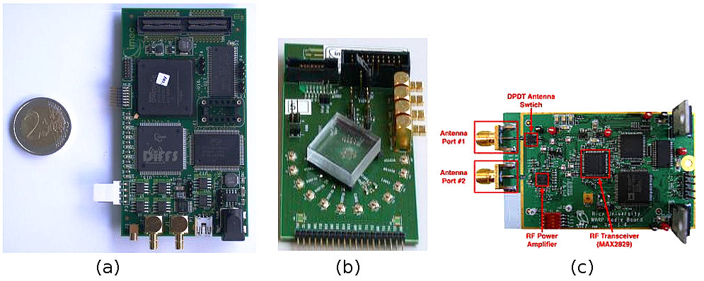
Figure 1 : Overview of boards for IMEC sensing engines deployted in CREW (a) SPIDER v2 digital board (b) Imec Scaldio-2B analog front-end (c) WARP analog front-end. A two Euro coin is shown to indicate the size of these boards.
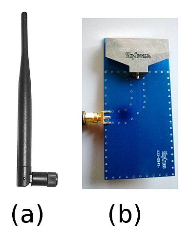
Figure 2 : example antenna's (a) Wifi antenna (b) broadband antenna for 800MHz .. 2.5 GHz range
| Attachment | Size |
|---|---|
| SPIDER-SCALDO2B-WARP.jpg | 112.92 KB |
| SE-antennas.jpg | 32.63 KB |
Software and hardware configuration
To use the IMEC sensing engine the hardware needs to be configured with the CREW API. The corresponding libraries are typically pre-compiled for the Zotac nodes of thw w-iLab.t test bed. Here we briefly illustrates the main configuration steps, as required when updating or extending nodes with Imec sensing capabilities. We show this for the default organisation of the development files, as illustrated in the user manual
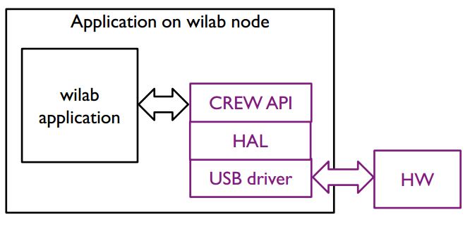
Figure 1 : software stack of the IMEC sensing engine
Software configuration
A high level overview of the software is shown in Figure 1. The software runs on Linux. The standard (lib)USB development kit implements the low level communication with the USB port on the SPIDER hardware board. An advantage of this approach is that the hardware abstraction layer (HAL), CREW sensing API (application programming interface) and application can be developed in user mode instead of kernel mode. The configuration is done as follows.
- Start up a terminal session
- Navigate to the top level directory of the development kit. You see two directories : "software" and "spider"
- cd spider/software/usb_interface/SensingEngine/ : this is the point where applications can be developed on top of the CREW sensing API
- source environment.csh : configure the environment with some additional variables
- pushd $USB_DIR : jump to directory with the spider HAL to communicate with the SPIDER board over USB
- make clean; make : build the spider API
- cd ../../platforms/swi/ : go to directory with the DIFFS HAL
- make clean ; make shared : build a shared library of the abstraction layer
- popd : jump back to the SensingEngine directory
- make clean ; make : build the CREW SensingEngine API
Hardware configuration
For CREW, the hardware configuration of the IMEC sensing engine is fixed. Two hardware configurations exist: one for systems equiped with a SCALDIO-2B front end, and another one when a WARP front-end board is present. In the spider/software/usb_interface/SensingEngine/ directory two scripts are available. Execute one of these to properly configure the SPIDER board:
- source environment.csh : only needed for a new terminal session
- ./setupscaldio.sh : execute this on nodes equiped with a Scaldio front end
- ./setupwarpfe.sh : execute this on nodes equiped with a WARP front end
With the command lsusb the hardware configuration can be checked. If the unitialised spider board is connected to the Zotac node, a USB device with ID 04b4:8613 of Cypress Semiconducor Corp. is present. After the hardware set-up this device is replaced by a USB device with ID 221a:0100. This signals that the SPIDER board is ready to use.
| Attachment | Size |
|---|---|
| SE-software-stack.JPG | 32.32 KB |
Program examples using the Imec sensing engine API
The Imec sensing engine is programmed in C, and can be set-up, configured and used with the sensing API. Using a simple example the use of this API is illustrated for the FFT_SWEEP mode. Both a single FFT sweep as multiple FFT sweeps are shown. This is illustrated for an Imec sensing engine equiped with a WARP front-end. A zip archive containing the source code of the examples is included below.
To conclude we provide an overview of the other modes as supported by the Imec sensing engine.
FFT_SWEEP example
The Imec sensing engine supports several modes: for this example uses FFT_SWEEP sensing scheme. This returns 128 points per selected channel. Figure 1 shows the output of one FFT sweep, for channel one to four for WARP, covering center frequencies 2412, 2432, 2452, 2472.
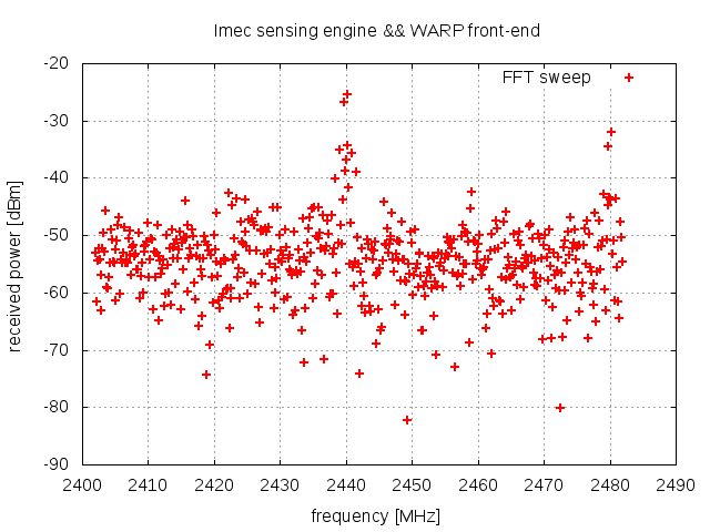
Figure 1 Output of one FFT sweep in the ISM band
The sensing engine is programmed in C. Items (1) .. (8) show the necessary steps to configure the sensing engine, and to produce the data shown in Figure 1. The full source code is available in the zip archive, specifically in the warp_single_FFT_SWEEP.c program file. In (9) we show how the program can be extended to do multiple sweeps.
The next paragraph discuss the required calls to the sensing API to produce the result.
Convention:
Type declarations are highlighted in green, and code snippets in blue. Calls to the sensing engine API are underlined.
1) Open the sensing engine handler
To open an Imec sensing engine board both the spider number and
front end number need to be used. The output is a software handler
that is used for the sensing engine API function calls.
se_t sensing_engine_handler;
sensing_engine_handler = se_open(spider, warp);
With:
- spider: an integer containing the spider board number. This number is bigger than 128 for spider v2 boards
- warp: a constant value 0 to select the WARP front end.
2) Initialize sensing engine
After checking the status of the sensing engine, the se_init function is
invoked to allocate memory and start adres for the my_se_config struct.
With this struct the parameters for the sensing engine will be configured.
A return value equal to 1 indicates that this step succeeded
int result = 0;
struct se_config_s my_se_config;
// configure WARP FFT sweep
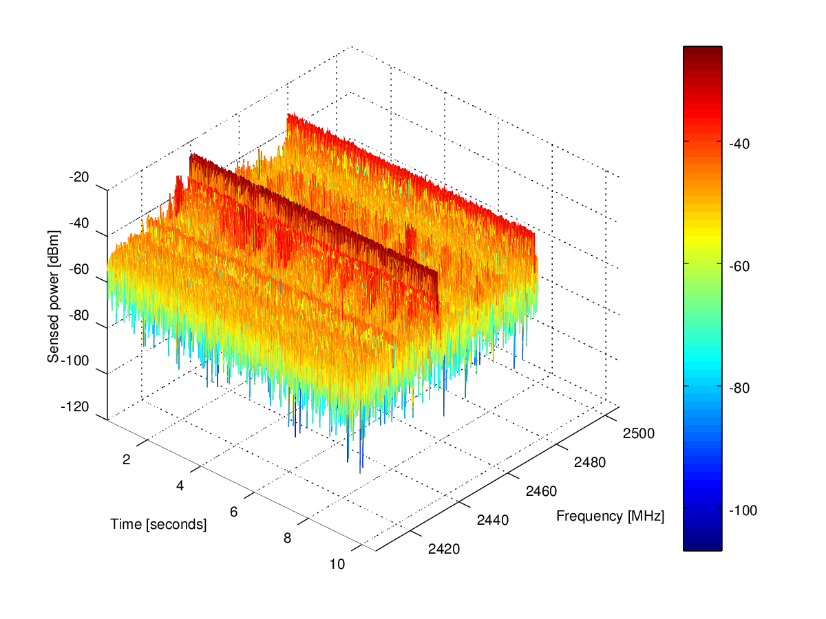
Other sensing modes
- FFT_SWEEP : shown in example above. A 128 point FFT is performed for each configured channel.
- WLAN_G: determines the instantaneous power in each selected channel for IEEE802.11g spectrum.
- WLAN_A: similar as WLAN_G, for IEEE802.11a spectrum.
- BLUETOOTH: determines instantanious power for IEEE802.15.1 spectrum.
- ZIGBEE: similar to BLUETOOTH, for IEEE802.15.4 spectrum
- LTE: not implemented.
- DVB_T: detection of DVB_T signals. Only applicable for the Scaldio2B front-end.
- ISM_POWER_DETECT: determines instantaneous power in the 2.4 GHz ISM band, with a granularity of 1 MHz.
- TRANSMIT: not implemented.
- ADC_LOG1: logging of ADC values as retrieved from the front-end. Debug mode for sensing engine equiped with a Scaldio2B front-end.
- ADC_LOG2: logging of ADC values as retrieved from the front-end. Debug mode for sensing engine equiped with a WARP front-end.
- STANDBY: not implemented.
| Attachment | Size |
|---|---|
| WARPexample.zip | 5.62 KB |
| Imec-sensing-engine-WARP-single-FFT-sweep.png | 10.84 KB |
| Imec-sensing-engine-WARP-multiple-FFT-sweep.png | 324.93 KB |
LOG-a-TEC documentation
All the documentation for the LOG-a-TEC testbed is now available here.
Common data format
Many cognitive usage scenarios that take place can be 'recorded'. In our federation data recorded in one testbed is usable in other testbeds to support emulated usage scenarios (e.g. primary user data recorded in testbed A feeds into a sensing device in testbed B).
To this end, CREW defined data of interest, common structures for storing data and is in the process of creating a federation database for storage of any collections made.
Information on the common data format can is available in this document. The corresponding tools that have been developed are available on GitHub by following this link.
| Attachment | Size |
|---|---|
| common-data-format.pdf | 327.93 KB |
Transceiver Facility Specification
The transceiver facility specification can be downloaded below.
"Fast Prototyping with WInnF Transceiver Facility Implementation for Fast Prototyping" project has been launched in the WInnF Transceiver System Interface Work Group (TSI-WG).
Link and text of where the source code can be found: WInnF where a C++ source code and its documentation is available.
| Attachment | Size |
|---|---|
| Transceiver_Facility_Specification-2009-01-28.pdf | 1.53 MB |
CREW benchmarking tools
This section explains the use of CREW benchmarking tools
The CREW benchmarking tools allow experimenters an easy setup, execution, and analysis of experiments that will be carried out on CREW federated testbeds. Currently, the tools are implemented in iMinds testbed and in short time it will be available to the other CREW testbeds. The tools are generic and easily portable to other testbeds with minor effort.
In order to be able to access to the CREW benchmarking tools running at the iMinds w-iLab.t Zwijnaarde testbed, a VPN account is needed. For information on how to obtain an account to w-iLab.t, please consult the following page.
CREW benchmarking tool list:
Easy experiment configuration
Tool Location (OpenVPN required) http://ec.wilab2.ilabt.iminds.be/CREW_BM/BM_tools/exprDef.html
The experiment definition tool allows the experimenter to configure the system under test and the wireless background environment. Two types of configuration are possible. One can start from scratch and create a full experiment definition or configure from an existing one.
For the latter case, a number of solution under test and background environment configuration files are stored in CREW repository.
For detail explanation, refer the section CREW experiment definition.
Experiment Definition Tool
The experiment definition tool is used to define, configure, and make changes to wireless experiments that are to be conducted on different testbeds. Before explaining the experiment definition in detail, an experimenter need to be familiar with the concept of experiment resource grouping. This concept is taken from the cOntrol and Management Framework (OMF) developed by the collaborative effort of NICTA and Winlab [1].
The experiment resource grouping concept treats an experiment as a collection of resources aggregated into groups. Resources can be any of these but not limited to WI-FI nodes, sensor nodes, spectrum sensing devices, and software-defined radios. With in a group, multiple nodes run different applications that were predefined in an application pool. And a single application as well defines a number of optional measurement points. In figure 1, we show a simple experiment scenario where two WI-FI nodes (node 1 and node 3) sends TCP and UDP packets towards two receiver WI-FI nodes (node 1 and node 3). In real life this could mean, for example, Node1 performing a file transfer to Node2 while at the same time listening to a high quality (192kbps) radio channel from Node3 and Node2 is watching a 10Mpbs movie streamed from Node3.
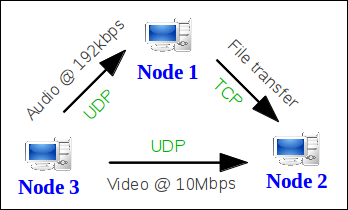
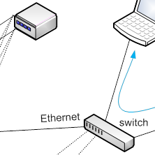
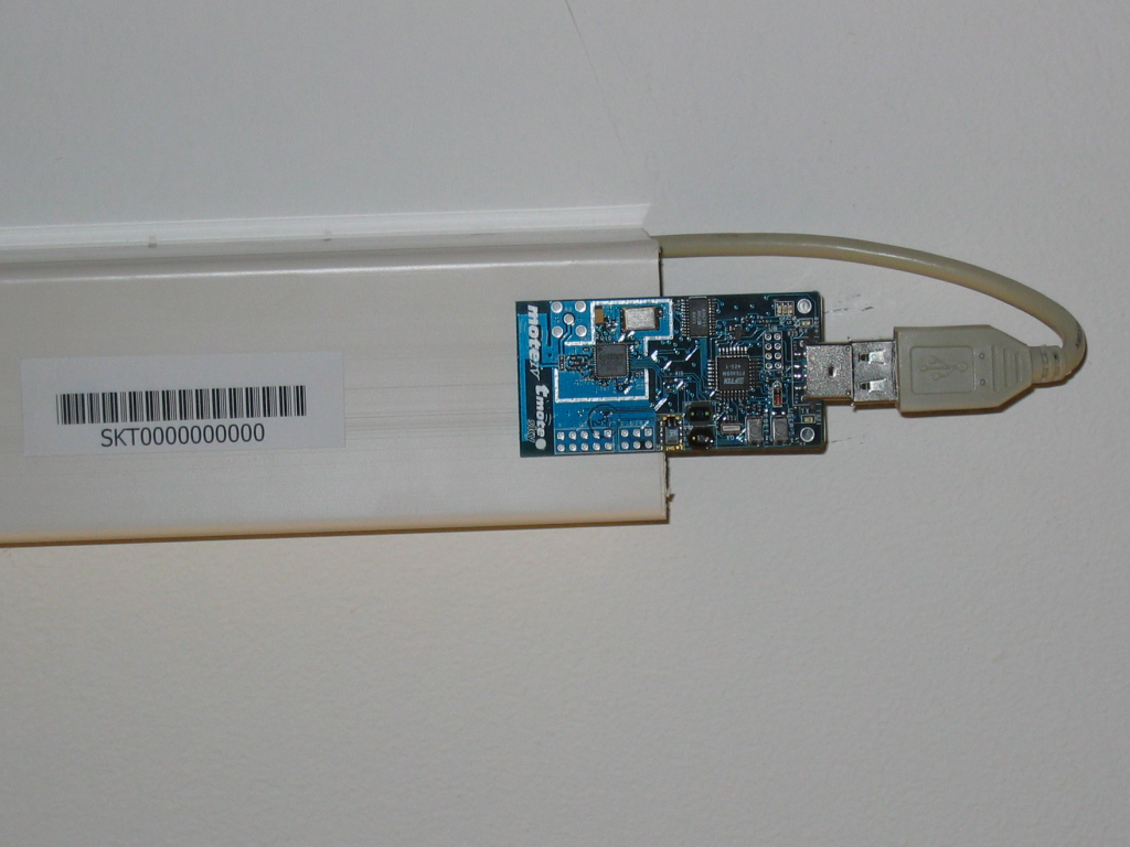
Figure 1. simple experiment scenario using three WI-FI nodes.
The experiment shown above, also called Iperf Sender Receiver (ISR) experiment , is realized using the iperf measurement tool which is a commonly used in network testing application. The iperf tool has a number of output formats instrumented for different uses. For example when iperf is used for TCP streaming, throughput information is displayed and when used for UDP streaming, jitter and packet loss information are displayed to the end user. Therefore an application can instrument more than one output to the user and in the context of OMF, they are refereed to as measurement points (MP). For this experiment scenario, transfer, jitter, and loss measurement points are used. A graphical view of experiment resource grouping is shown in figure 2.
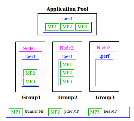
Figure 2. Experiment resource grouping of the experiment scenario. Note that Node3 does not have measurement points since it only streams UDP packets.
Next we look at how experiment is defined in the experiment definition tool. The ISR experiment, defined previously, is used here to illustrate tool's usage. From an experimenter point of view, there are two ways of defining an experiment. These are defining new experiment and defining from a saved configuration file.
Click the Start New Configuration link to start defining a new experiment. The first stage of experiment definition is experiment abstract. Here the experimenter can give a high level information about the experiment such as project name, experiment name, title, author, contact information, summary, and duration. Figure 3 shows the experiment abstract of the ISR experiment.
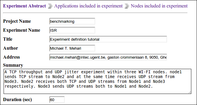
Figure 3. Experiment abstract definition of ISR experiment.
The next step is application definition. Here we create the application pool containing all applications that will be used in the experiment. Figure 4 shows the iperf application from ISR experiment application pool.
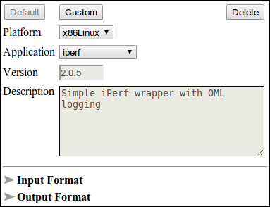
Figure 4. iperf application defined inside the application pool.
The last step in experiment definition tool is binding applications from the pool to different nodes of the wireless testbed. It involves platform specific node selection from testbed layout, interface configuration of group of nodes, and finally binding applications to nodes. Application binding involves a number of steps which are application selection, optional output instrumentation, input parameter configuration, and application timeline definition. Figure 5 shows the node configuration section (only shown for group Node1) of the ISR experiment.
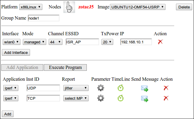
Figure 5. Experiment node configuration of ISR experiment.
Finally after finish configuring the experiment definition, we save it to a configuration package (name it ISR) composed of three files. These are XML configuration file (ISR.xml), OEDL (OMF Experiment Description Language) file (ISR.rb), and a network simulation file (ISR.ns) containing all configuration setting to be used inside emulab framework [2]. We explain the content of the XML configuration file in this section but the rest two files are explained on a separate page.
In CREW, XML is used as a configuration format for experiment descriptions and the XML configuration of the experiment definition in particular is a subset of the CREW common data format. An overview of the XML configuration of the ISR experiment is shown in figure 6.
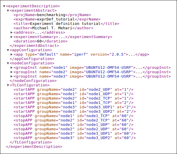
Figure 6. Excerpt from ISR experiment XML configuration file
Defining an experiment from a saved configuration file
For the experimenter, defining everything from scratch might be time consuming. An experimenter can use an existing configuration file or customize it according to his need. Reconfiguration is done first by downloading the configuration file (look CREW repository, background environments section in CREW portal) and then loading it on the "Load/Configure Experiment" section of the experiment definition tool. Finally, start reconfiguration and save it after finish modification.
[1]. Thierry Rakotoarivelo, Guillaume Jourjon, Maximilian Ott, and Ivan Seskar, ”OMF: A Control and Management Framework for Networking Testbeds.”
Configure parameters, provision and run experiments
Tool Location (OpenVPN required): http://ec.wilab2.ilabt.iminds.be/CREW_BM/BM_tools/exprExec.html
Experiment Execution Tool
Recall at the end of CREW experiment definition tool, we end up with a tar package containing three different files. The first file, ISR.xml, is an XML experiment description file for the ISR experiment. The second file generated, ISR.rb, is an experiment description of the type OEDL (OMF Experiment Description Language) and the last file generated, ISR.ns, is a network simulation file containing all configuration settings to be used inside emulab framework. Current implementation of the CREW experiment execution tool only works on top of OMF (cOntrol and Management Framework) testbeds. But it is designed to be versatile and work with different testbeds having their own management and control framework. The tool interacts with the testbed using a specific API designed for the testbed. Thus working on a different testbed with a different framework only relies on the availability of interfacing APIs and minor change on the framework itself.
Coming back to what was left at the end of the experiment definition tool, we start this section by using the two files generated (i.e. ISR.rb and ISR.ns). Details of the ISR.rb file and OEDL language are described on a separate page. However, to have a deeper understanding of the language details, one can study OEDL 5.4.
We start by definining the experiment topology on the emulab framework [1] using the NS file ISR.ns. Tutorial about creating your first experiment on the emulab framework and explanation of the NS file follows this page. After finish defining your topology and swapping in your experiment in the emulab framework, start the experiment execution tool. The experiment execution tool allows experimenters load an experiment description, configure parameters, schedule, and finally start an experiment. Figure 1 shows the front view of the experiment execution tool after the OEDL file (i.e. ISR.rb) is loaded.
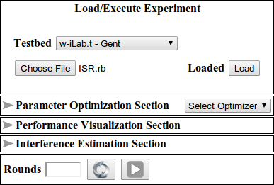
Figure 1. Experiment execution tool at glance.
After loading the file, four different sections are automatically are populated and each section performs a specific task.
- Parameter Optimization Section configures single/multi dimensional optimizer that either maximizes or minimizes an objective performance.
- Performance Visualization Section configures parameters to be visualized during experiment execution.
- Interference Estimation Section configures the pre/post interference estimation of experiments and detect unwanted wireless interference that could influence the experiment.
- Experiment Rounds section configures the number of identical runs an experiment is executed.
Recall the scenario of ISR experiment where Node 1 performs a file transfer to Node 2 while at the same time listening to a high quality (192kbps) radio channel from Node 3 and Node 2 is watching a 10Mbps movie stream from Node 3.
Now starting from this basic configuration, let us say we want to know how large the video bandwidth from Node 3 to Node 2 can increase so that we see a high definition movie at the highest possible quality. This is an optimization problem and next we see how to deal with such a problem using the experiment execution tool.
- Select IVuC optimizer from the Parameter Optimization section and click the text on the left side to reveal its content.
- Select Node3_UDP2_bandwidth as design space parameter located at the end of the Tune list.
- Start from 10,000,000 bps using step size 2,000,000 bps and reduction rate of 0.5. The optimizer either stops once the step size is reduced to 100,000 bps or when search parameter exceeds 20,000,000 bps.
- In the objective variables subsection, configure two variables to calculate the sending and receiving bandwidth using the aggregation AVG.[ Note: Click the plus icon on the right hand corner to add extra variables]
- Define your objective function as a ratio of the two variables (i.e. (8*x1)/x2) defined previously and select the condition less than with a stopping criteria 0.95 (i.e. (8*x1)/x2 < 0.95 => Stop when 8*x1 < 0.95*x2). [ Note: The reason 8 is multiplied to x1 variable is because iperf reports bandwidth in byte/sec].
Figure 2 shows the configuration details of parameter optimization section.
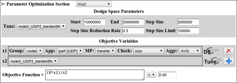
Figure 2. IVuC optimizer configuration for the ISR experiment.
The next thing we do is configure the performance visualization section where we define parameters to be visualized during experiment execution. For this exercise, we visualize the UDP and TCP bandwidth performance at Node2 coming from Node3 and Node1 respectively. As the wireless medium is shared among all Nodes, the UDP bandwidth stream from Node3 is affected by the TCP bandwidth stream from Node1 and visualizing these two parameters reveal this fact. Figure 3 shows the configuration detail of performance visualization section.
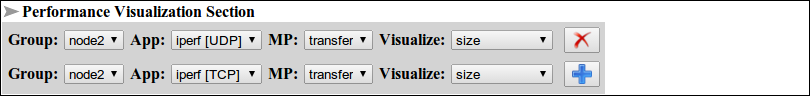
Figure 3. Performance visualization configuration for the ISR experiment
After that, we can enable interference estimation and check for possible pre and post experiment interferences. This is one way of detecting outlier experiments as there is a higher possibility for experiments to be interfered if the environment before and after their execution is interfered. For now, we skip this section. Similar to the experiment definition tool, execution configuration settings can be saved to a file. Click the button  to update the execution configuration into the OEDL file and later reloading the file starts the experiment execution page pre configured. Finally, set the number of experiment rounds to one and click on the button
  .
.
Once the experiment has started, the first thing we see is a log screen populated with debug information. The debug information contains high level information about the experiment such as defined properties, experiment ID, events triggered, and a lot more. The log screen view being an important interaction tool to the experimenter, there is also a second view called the graph screen view. To switch to the graph screen view, click the notebook icon  from the experimentation screen. The graph screen view displays parameters that were defined in the performance visualization section (see above) as a function of time. For the ISR experiment, the UDP and TCP bandwidth plot as a function of time from node3 and node1 are displayed respectively. Figure 4 shows the graph screen view of the ISR experiment.
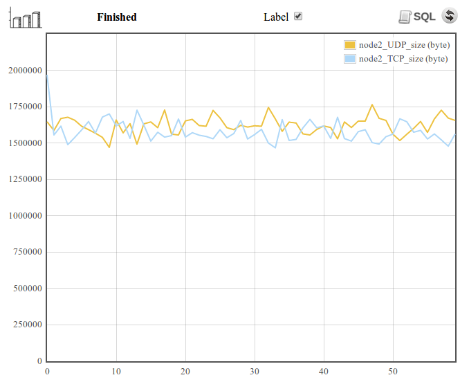
Figure 4. A glance at the graph screen view from experimentation screen.
From the above figure, we note a couple of things. Top on the left, there is the graph icon which triggers the debug information view up on clicking. Next is the experiment status (i.e. Scheduled, Running, Finished) indicator. The label check box turns the label ON and OFF. Execution of SQL statements is allowed after the experiment has stopped running. SQL statements are written in the log file viewer by which switching to this view, writing your SQL statements and pressing the icon  executes your statements. Finally the UDP and TCP bandwidth as a function of time are plotted and it also indicates an equal bandwidth share between both applications. Not shown on the figure but also found on the experimentation screen are parameter settings, objective value, correlation matrix table, and experiment run count.
Following the whole experimentation process, we see the ObjFx. Value (i.e. (8*x1)/x2) starts around 1 and decreases beyond 0.95 which triggers the second experimentation cycle. The optimization process carries on and stops when step size of Node3_UDP2_bandwidth reaches 100,000 bps. The whole process takes around 11 minutes under normal condition. The IVuC optimizer locates an optimal bandwidth of 14.125 Mbps UDP traffic from Node3 to Node2. Therefore the highest bit rate a movie can be streamed is at 14.125 Mbps.
Finally, the experimenter has the option to save experiment traces and later perform post processing on the stored data. CREW also incorporates a post processing tool to facilitate benchmarking and result analysis. The aim of this tool is to make comparison of different experiments through graph plots and performance scores. A performance score can be an objective or a subjective indicator calculated from a number of experiment metrics. The experiments themselves doesn't need to be conducted on a single testbed or with in a specific time bound, as long as experiment scenarios (aka experiment meta data) fit in the same context. Thus an experiment once conducted can be re-executed at a latter time in the same testbed or executed on a different testbed and conduct perform comparison of the two solutions.
For this tutorial save the experiment (i.e. press the Save experiment result button) by giving a name (e.g. Solution_one) and start post processing on the saved data using the benchmarking and result analysis tool. Please be reminded that only selected experiment runs are saved to a file and you should tick the check box next to each experiment run that you want to save.
List of optimizers explained
Experiment optimization is the heart of the CREW experiment execution tool. The efficiency of an experiment execution tool mostly depends on how it optimizes the different experiments to come and how fast it converges to the optimum. However, due a variety of problems in the real world, coming up with a single optimizer solution is almost impossible. The normal way of operation is to categorize similar problems into groups and apply unique optimizers to each one of them. To this end, the experiment execution tool defines a couple of optimizers which are fine tuned to the needs of most experimenters. Thus this paper explains the working principle of each optimizer supported in the experiment execution tool.
Step Size Reduction until Condition (SSRuC) optimizer
SSRuC is a single parameter optimizer aimed at problems which show local optimum or local minimum in the vicinity of the search parameter. Such kinds of problems are approximately described using two monotonically increasing and decreasing functions from either side of the optimum point. Figure 1 explains the problem graphically.
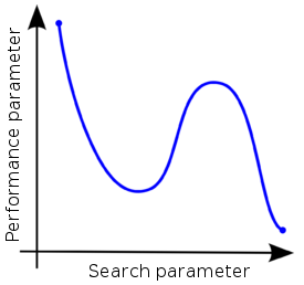
Figure 1. An example showing two local optimas with monotonic functions on either side of the optimum points
SSRuC tackles such problems using the incremental search algorithm approach [1]. Five parameters are passed to the optimizer. These are the starting, ending, step size of the search parameter, the step size reduction rate and the step size limit used as a stopping criteria by the optimizer. The optimizer starts by dividing the search parameter width into fixed intervals and performs unique experiment at each interval. For each experiment, measurement results are collected and performance parameters are computed. Next, a local maximum or local minimum is selected from performance parameters depending on the optimization context. If the optimization context is "maximization", we take the highest score value whereas for "minimization" context, we take the lowest score value. After that, a second experimentation cycle starts this time with a smaller search parameter width and step size. The experimentation cycle continues until the search parameter step size lowers below the limit. Figure 2 shows the different steps involved.
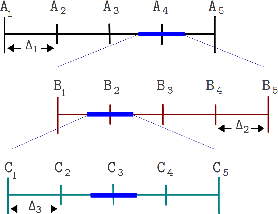
Figure 2. The different steps involved in an SSRuC optimizer over the search parameter width A1 to A5
Figure 2 shows the SSRuC optimizer in a three level experimentation cycle. In the first cycle, five unique experiments are conducted out of which the fourth experiment (experiment A4 ) is selected. The second experimentation cycle works in the neighborhood of A4 with a reduced step size ?2 . This cycle again conducts 5 unique experiments out of which the second experiment (experiment B2 ) is selected. The last experimentation cycle finally conducts 5 unique experiments from which the third experiment (experiment C3) is selected and treated as the optimized value of the parameter.
Increase Value until Condition (IVuC)
IVuC optimizer is designed to solve problems which show either increasing or decreasing performance along the design parameter. A typical example is described in the experiment execution tool where video bandwidth parameter was optimized for a three node Wi-Fi experiment scenario. Datagram error rate was set as a performance parameter and the highest bandwidth was searched limited to 10% datagram error rate and below.
The algorithm used by IVuC optimizer is similar to the SSRuC optimizer in such a way that both rely on incremental searching. However, the main difference between the two is that the SSRuC optimizer performs a complete experimentation cycle before locating the local optimum value whereas the IVuC optimizer performs a local optimum performance check after the end of each experiment. Later on, both approaches refine their searching parameter range and restart the optimization process to further tune the search parameter. Figure 3 shows the different steps involved in IVuC optimizer.
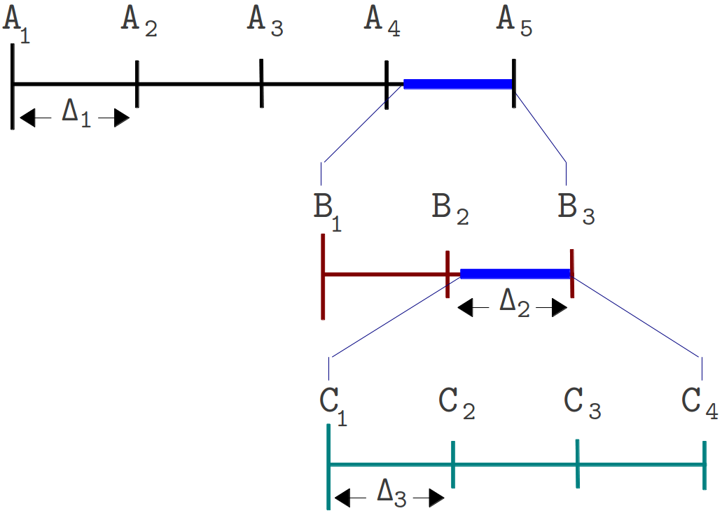
Figure 3. The different steps involved in an IVuC optimizer over the search parameter width A1 to A5
From figure 3, we see the three experimentation cycles each with five, three, and four unique experiments respectively. At the end of each experimentation cycle, performance parameter drops below threshold and that triggers the next experimentation cycle. At the end of the third experimentation cycle, a prospective step size ?4 was checked and found below threshold, making C4 the optimal solution.
Unlike SSRuC and IVuC, SUMO optimizer works on multiple design parameters and multiple design objectives. It is targeted to achieve accurate models of a computationally intensive problem using reduced datasets. SUMO manages the optimization process starting from a given dataset (i.e. initial samples + outputs) and generates a surrogate model. The surrogate model approximates the dataset over the continuous design space range. Next it predicts the next design space element from the constructed Surrogate model to further meet the optimization’s objective. Depending on the user’s configuration, the optimization process iterates until conditions are met.
The SUMO optimizer is made availabe as a MATLAB toolbox and works as a complete optimization tool. It bundles both the control and optimization functions together where the control function sitting at the highest level manages the optimization process with specific user inputs. Figure 4 shows SUMO toolbox in a nutshell highlighting the control and optimization functions together.
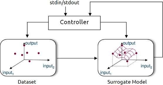
Figure 4. Out of the box SUMO toolbox in a nutshell view
In the context of CREW benchmarking tools, the aim is to use SUMO toolbox as a standalone optimizer and put it inside the experimentation framework. This means starting from out of the box SUMO toolbox, the loop is broken, the control function is removed and clear input/output interfaces are created to interact with the controlling framework. Figure 5 shows how modified SUMO toolbox is integrated in the wireless testbed.
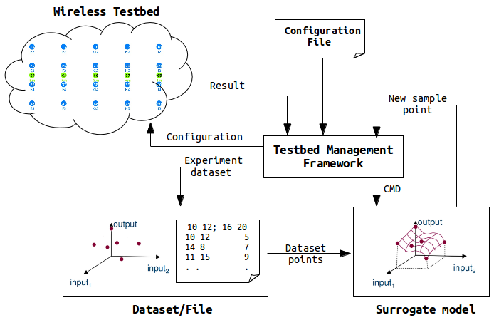
Figure 5. Integration of SUMO toolbox in a wireless testbed
The testbed management framework in the above figure controls the optimization procdess and starts by executing a configuration file. The controller pases configurations and control commands to the wireless nodes and measurement results are send back to the controller. After executing a number of experiments, the controller starts the SUMO toolbox supplying the experiment dataset which has been executed so far. The SUMO toolbox creates a surrogate model from the dataset and returns the next sample point to the controller. The controller again executes a new experiment with the newest sample point and generates a new dataset. Next the controller calls the SUMO toolbox again sending the dataset (i.e. one more added). The SUMO toolbox creates a more accurate surrogate model with the addition of one dataset. It sends back a new sample point to the controller and the optimization continues until a condition is met. It should be understood, however, that operation of the customized SUMO toolbox has not changed at all except addition of a number of blocks.
Having said about its operation, an example of wireless press conference optimization using customized SUMO toolbox is located on this link.
[1]. Jaan Kiusalaas, ”Numerical Methods in Engineering with MATLAB” Cambridge University Press, 01 Aug 2005, pp 144-146.
OEDL explained
This section provides a detailed description of the experiment description file, ISR.rb, that was created during the hands on tutorial on experiment definition tool. It mainly focus on introducing the OEDL language, the specific language constructs used inside ISR.rb file, how it is mapped to the XML experiment description file, and finally a few words on the tools OEDL language capability.
OEDL (OMF Experiment Description Language) is a Ruby based language along with its specific commands and statements. As a new user, it is not must to know the Ruby programming language. And with a simple introduction on the language, one can start writing a fully functional Experiment Description (ED) file. Any ED file written in OEDL is composed of two parts
- Resource Requirements and Configuration: this part enumerates the different resources that are required by the experiment, and describes the different configuration to be applied.
- Task Description: this part is essentially a state-machine, which enumerates the different tasks to be performed using the requested resources.
This way of looking an ED file is a generic approach and basis for learning the OEDL language. But specific to this tutorial we take a different approach and further divide content of an ED file into three sections.
Application Definition section
This section of ED file, all application resources taking part in the experiment are defined. Each application defines specific properties like input parameters, measurement points, and application specific binaries. Figure 1 shows an excerpt of the application definition from ISR.rb file.
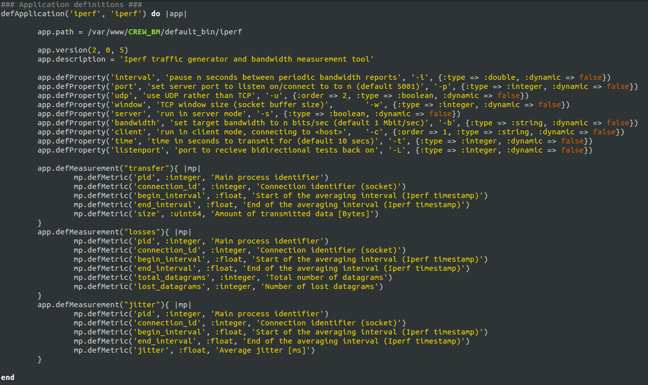
Figure 1. excerpt of ISR.rb application definition
From figure 1, we see a number of OEDL specific constructs. The defApplication command is used to define a new application. Such defined application can be used in any group of nodes as required. The defProperty command defines an experiment property or an application property. Experiment property is a variable definition that can be used anywhere inside the OEDL code. For example node1_UDP_server and node1_UDP_udp are two property definitions inside ISR.rb file. Application property on the other hand is defined inside an application and can only be accessed after the application is added. For example interval, port, udp, and others are application properties of iperf program. Next is the defMeasurement command used to define a single Measurement Point (MP) inside an application definition. Finally the defMetric command defines different output formats for the given MP.
Group Definition section
In the group definition, a group of nodes are defined and combined with the applications defined earlier. Figure 2 shows an excerpt of ISR.rb file group definition only for Node1.
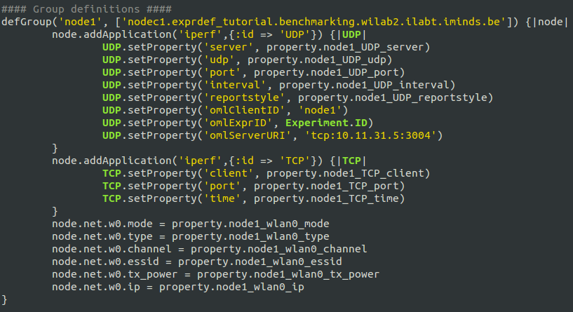
Figure 2. excerpt from iperf group definition in ISR.rb file
In this section, a number of OEDL specific constructs are used. The first one is defGroup which is used to define group of nodes. Here only nodeC1 from the testbed is defined inside the group Node1. addApplication is the second command used and it adds application into the group of nodes from the application pool. Since it is possible to add a number of identical applications with in a single group, it is good practice to give unique IDs to each added application. For the Node1 group, two iperf applications are added with IDs TCP and UDP. setProperty command is used to set values to different input parameters of the application added. Finally node specific interface configuration is handled by resource path constructs. For the Node1 group mode, type, channel, essid, tx_power, and ip configurations are set accordingly.
Timeline Definition section
The timeline definition defines the starting and stopping moments of each defined applications with in each group of nodes. Figure 3 shows an excerpt of ISR.rb file timeline definition.
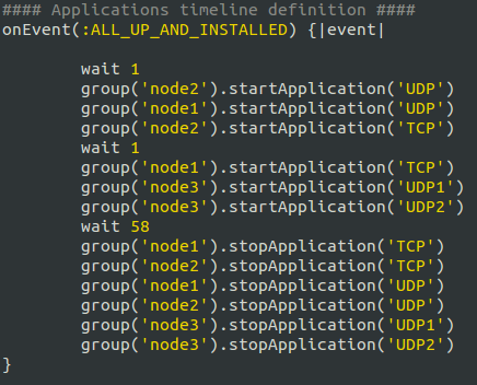
Figure 3. excerpt from iperf timeline definition in ISR.rb file
Inside OEDL language, events play a huge role. An Event is a physical occurrence of a certain condition and an event handler performs a specific task when the event is triggered. ALL_UP_AND_INSTALLED event handler shown in figure 3, for example, is fired when all the resources in your experiment are requested and reserved. The wait command pauses the execution for the specified amount of seconds. Starting and stopping of application instances are executed by the commandstartApplication and stopApplication respectively. Application IDs are used to start and stop specific applications. For example group('node1').startApplication('UDP') refers to the application iperf from node1 group with ID UDP.
So far we walk you through the default OEDL constructs that are used throughout the ISR.rb file. It is also possible to define custom OEDL constructs and one such use is custom event definition. We used custom event definition in our ISR.rb file to check if all applications are stopped. If so we trigger the EXPERIMENT_DONE event and end the experiment execution. Figure 4 shows the custom event definition used inside ISR.rb file.
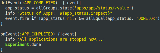
Figure 4. custom event definition section in ISR.rb file
We create a custom event using the command defEvent. By default custom defined events are checked every five seconds for possible event triggering. Inside the event definition, we wait until all applications are finished and fire the event handler afterwards. The event handler is defined following the onEvent commandpassing name of the event definition APP_COMPLETED. Finally when the event is triggered, the handler calls the EXPERIMENT_DONE method which stops the experiment execution and releases all allocated resources.
Mapping OEDL to XML experiment description
Recall from experiment definition tool section that an experimenter passes three steps to finish configuring its experiment and produce XML, OEDL, and ns files. It is hidden to the experimenter however that an OEDL file is generated from the XML file. During the making process of configuration package, an XML template is first produced out of which the OEDL file is constructed.
The mapping of OEDL to XML is straight forward. It follows a one to one mapping except rearrangement of text. The following three figures show a graphical mapping of XML to OEDL on application definition, group definition, and timeline definition sections accordingly.
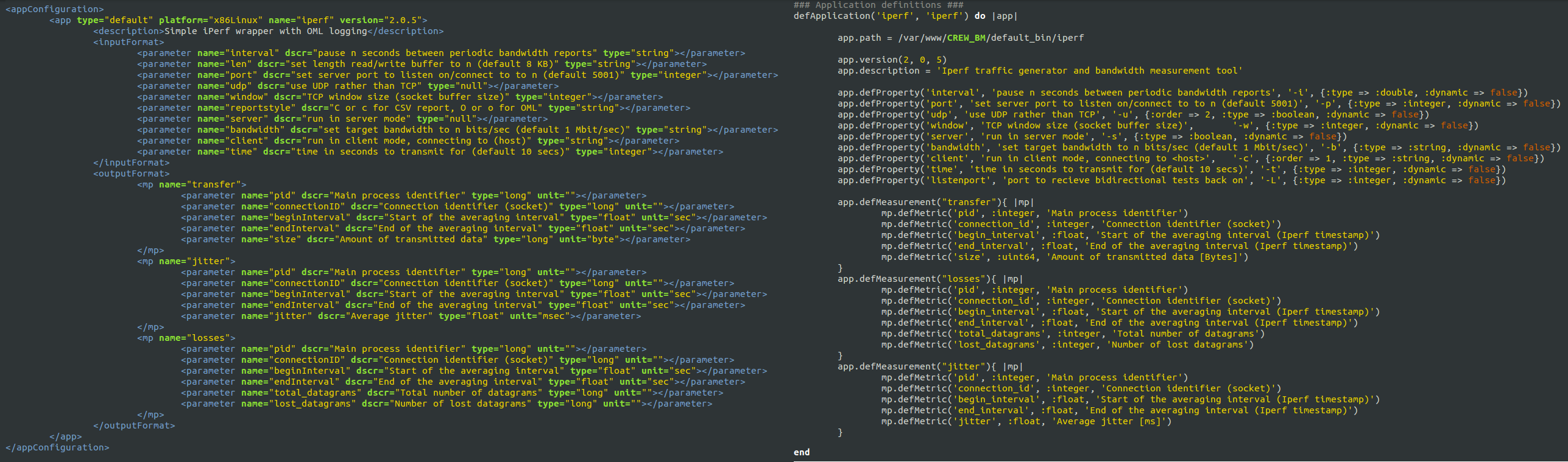
Figure 5. XML to OEDL application definition mapping inside ISR.rb file
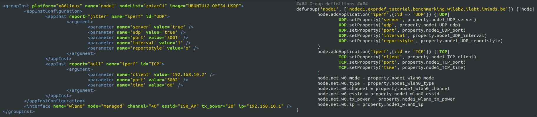
Figure 6. XML to OEDL group definition mapping inside ISR.rb file
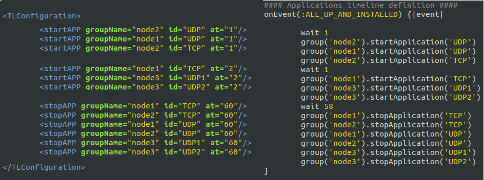
Figure 7. XML to OEDL timeline definition mapping inside ISR.rb file
Wireless press conference optimization using SUMO toolbox
Problem Statement
A wireless press conference scenario comprises of a wireless speaker broadcasting audio over the air and a wireless microphone at the listner end playing the audio stream. This type of wireless network is gaining attention specially in a multi-lingual conferencing room where the speaker's voice is translated into different language streams and broadcasted to each listner where they select any language they want to hear the translated version. However the wireless medium is a shared medium and it is possible to be interfered by external sources and we want to optimize the design parameters which gives the best audio quality. Moreover, we also want to reduce the transmission exposure which is a direct measure of electromagnetic radiation. Transmission exposure is gaining attention these days related to health issues and regulatory bodies are setting limits on maximum allowable radiation levels. Thus our second objective is to search design parameters that lowers transmission exposure of the wireless speaker exposed on each listner. For this tutorial, two design parameters of the wireless press conference are selected (i.e. transmit channel and transmit power) and we optimize these parameters inorder to increase the audio quality and decrease transmission exposure.
Experiment scenario
The experiment is composed of one speaker and 5 listeners making the Solution Under Test (SUT) and one public access point creating a background interference. The public access point is connected to three WI-FI users and provides a streaming video service at the time. Figure 1 shows the experiment scenario.
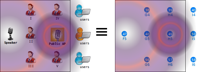
Figure 1. Experiment scenario of 5 listners, 1 speaker , 1 public access point, and 3 users.
On the left hand side, the realistic press conference scenario is shown. On the right hand side, the experimentation scenario as seen on the w.ilab.t zwijnaarde testbed [1] is shown. The horizontal and vertical distances between consecutive nodes is 6m and 3.6m respectively. All listener nodes (i.e. 38, 39, 48, 56, and 57) are associated to the speaker access point (i.e. node 47). Background interference is created by the public access point (i.e. node 49) transmitting on two WI-FI channels (i.e. 1 and 13) at 2.4Ghz ISM band.
The wireless speaker, configured on a particular transmit channel and transmit power, broadcasts a 10 second WI-FI audio stream and each listener calculates the average audio quality within the time frame. The wireless speaker at the end of its speech averages the overall audio quality from all listeners and makes a decision on its next best configuration. The wireless speaker using its newest configuration again repeats the experiment and produces a second newest configuration. This way the optimization process continues iterating until conditions are met.
The public access point on the other side transmits a 10 Mbps continuous UDP stream on both channels (i.e. channel 1 and 13) generated using iperf [2] application. In the presence of interference, audio quality gets degraded and the wireless speaker noticing this effect (i.e. lower audio quality) has two options to correct it. Either increase the transmission power or change the transmission channel. Making the first option is unlikely because it increases the transmission exposure. Changing the transmission channel also has limitations; the problem of overlapping channels interference [3]. Overlapping channels interference results in quality degradation much worse than identical channel interference. In identical channel interference, both transmitters apply CSMA-CA algorithm and collision is unlikely to happen. However in overlapping channels interference, transmitters don’t see each other and collision likely happens.
Two fold optimization
As was explained previously, we want to optimize the design parameters that brings an increased audio quality and decreased transmission exposure. A straight forward solution is to perform unique experiments at each design parameter combinations also known as exhaustive searching and locate the optimum design parameters which gives the highest combined objective (i.e. audio quality + transmission exposure).
Audio quality objective
In the earlier telephony system, Mean Opinion Score (MOS) was used for testing audio quality out of a 1 to 5 scale (i.e. 1 for the worst and 5 for the best quality). MOS is a subjective quality measure that no two people give the same score. However due to recent demands in Quality of Service (QoS), subjective scores are replaced by objective scores for the reason of standardization. Moreover, the earlier telephony system is now replaced by the more advanced Internet Protocol (IP) driven backbones where Voice over IP (VoIP) service becomes the prefered method of audio transportation.
In a VoIP application, audio quality can be affected by a number of factors. Amongst all packet loss, jitter, and latency take the most part. An objective quality measure based on these parameters is standardized as ITU-T PESQ P.862. A mapping of PESQ score to MOS scale is presented in [4]. Here packet loss, jitter, and latency are measured for a number of VOIP packets arriving at the receiver end. Averaging over arrived number of packets, jitter and latency are combined to form an effective latency which also considers protocol latencies. Finally, the packet loss is combined to effective latency in a scale of 0 to 100 called the R scale. Finally the R scale is mapped to 1 to 5 scale and MOS score is generated. Figure 2 shows the pseudo code excerpt of MOS calculation.
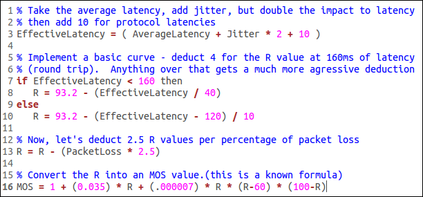
Figure 2. MOS score calculation code excerpt
Tranmission exposure objective
Transmission exposure is a direct measure of the electric-field strength caused by a transmitter. In [5] an in depth calculation of transmission exposure is presented. Exposure at a certain location is a combined measure of radiated power, transmitted frequency and path loss. Now a days regulatory bodies are setting maximum allowable exposure limits in urban areas. For example Brussels, captial city of Belgium, sets transmission exposure limit to 3v/m.
Characterizing the exposure model requires calculation of the path loss model specific to the experimentation site. The experimentation site at our testbed has a reference path loss of 47.19 dB at 1 meter and path loss exponent 2.65. Having this measurement, transmission exposure is calculated for each participating nodes and later average the sum over the number of nodes. Figure 3 shows the average exposure model.
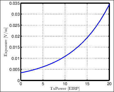
Figure 3. Average transmission exposure
Exhaustive searching optimization
The exhaustive searching optimization performs in total 13 channels x 20 TxPower = 260 experiments. Figure 4 and 5 shows performance output of the exhaustive searching optimization.
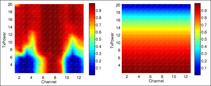
Figure 4. Audio quality and exposure global accurate model with background interference at channels 1 and 13
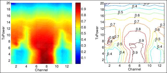
Figure 5. Dual objective and contour global accurate model with background interference at channels 1 and 13
The dual objective model shown in figure 5 is combined from the audio quality and exposure models shown in figure 4. Looking into the audio quality model, areas with a higher transmission power have good performance in general. However, there is an area on the non-interfered channel (i.e. 6 to 8), where there is a sudden jump in performance as TxPower increases from 4 dBm to 8 dBm. This area is of interest to us where higher audio quality and lower transmission exposure are seen. Indeed this is shown as a dark red region in the dual objective global accurate model.
Another aspect to look is the area where worst performance is recorded. Look again on the left side of figure 5 between channels 2 to 4, 10 to 12 and TxPower 1 to 7. Interestingly, this region is not located on channels where background interference is applied on but on its neighboring channels. This is due to the fact that the speaker and interferer nodes apply CSMA-CA algorithm on identical channel but not on neighboring channels which results in worst performance [3].
Note: TODO
Click the different areas on figure 4 to hear the audio quality when streamed at the specific design parameters
SUMO toolbox optimization
The exhaustive searching optimization gives the global accurate model however it takes very long time to finish the experimentation. Now we apply SUMO toolbox to shorten the duration and yet achieve a very close optimum value compared to the global accurate model shown in figure 5.
Start experiment execution using the preconfigured files located at the end of this page. The optimization process starts by doing 5 initial experiments selected using Latin Hypercube Sampling (LHS) over the design parameter space. LHS selects sample points on the design space evenly and with minimum sample points it assures providing the best dynamics of the system. For each of the five intial sample points, combined objectives are calculated which forms the inital dataset. The SUMO toolbox reads the inital dataset, creates a surrogate model out of it, and provide the next sample for experimentation to be carried on. The iteration continues until the stopping criteria is met. The stopping criteria selected, at the end of every iteration, sorts the collected combined design objective in ascending order and take the last five elements. Next calculate the standard deviation of this list and stop iteration when the standard deviation falls below threshold. A threshold of 0.05 is selected such that it is twice the standard deviation of a clean repeatable experiment [6]. The idea behind choosing such criteria is that the output of a sorted experiment approaches a flat curve as the optimization reaches the optimum. And the sorted last few elements show a small standard deviation.
Three sets of experiments are conducted and the results are compared to the global accurate model interms of Performance Gain (PG) and Duration Gain (DG) metrics. figure 7 shows the plot of sorted last 5 iteration standard deviation as a function of iteration/duration gain until stopping criteria (i.e. STD_MIN < 0.05) is met.
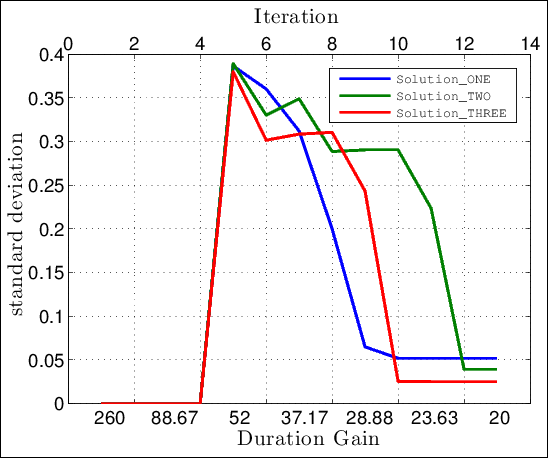
Figure 7. sorted last 5 iterations standard deviation plot
Shown in the figure above, all solutions stop execution around the 12th iteration (i.e. DG=21.5). Their perfomance gain compared to the global accurate model gives
Solution_ONE PG = [Solution optimum]/[Global accurate optimum] = -0.8261/-0.8482 = 0.9739
Solution_TWO PG = [Solution optimum]/[Global accurate optimum] = -0.8373/-0.8482 = 0.9871
Solution_THREE PG = [Solution optimum]/[Global accurate optimum] = -0.8352/-0.8482 = 0.9846
From the above results we conclude that by applying SUMO toolbox to wireless press conference problem, we improved the optimization process around 21.5 faster than the exhaustive searching optimization. And yet their performance is almost identical.
[1] http://www.ict-fire.eu/fileadmin/events/2011-09-2OpenCall/CREW/Wilabt_crewOpenCallDay.pdf
[2] Carla Schroder, ”Measure Network Performance with iperf” article published by Enterprise Networking Planet, Jan 31, 2007
[3] W. Liu, S. Keranidis, M. Mehari, J. V. Gerwen, S. Bouckaert, O. Yaron and I. Moerman, "Various Detection Techniques and Platforms for Monitoring Interference Condition in a Wireless Testbed", in LNCS of the Workshop in Measurement and Measurement Tools 2012, Aalborg, Denmark, May 2012a
[4] http://www.nessoft.com/kb/50
[5] D. Plets, W. Joseph, K. Vanhecke, L. Martens, “Exposure optimization in indoor wireless networks by heuristic network planning”
[6] M. Mehari, E. Porter, D. Deschrijver, I. Couckuyt, I. Morman, T. Dhaene, "Efficient experimentation of multi-parameter wireless network problems using SUrrogate MOdeling (SUMO) toolbox", TO COME
| Attachment | Size |
|---|---|
| audioQltyExpOptSUMO.tar | 1.9 MB |
Process and check quality
Show and compare results
Tool Location (OpenVPN required): http://ec.wilab2.ilabt.iminds.be/CREW_BM/BM_tools/exprBM.html
The benchmarking and result analysis tool is used to analyze results obtained and benchmark the solution by comparing it to other similar solutions. As the name implies, the tool provides result analysis and score calculation (aka benchmarking) services. In the result analysis part, we do a graphical comparison and performance evaluation of different experiment metrics. For example, application throughput or received datagram from two experiments can be graphically viewed and compared. In score calculation part, we do advanced mathematical analysis on a number of experiment metrics and come up with objective scores.
Benchmarking and result analysis
Most of the time the steps involved in wireless experimentation are predefined. Start by defining an experiment, execute the experiment, analyze and compare the result. This tutorial explains the last part which is result analysis and performance (aka score) comparison. In the result analysis part, different performance metrics are graphically analyzed. For example, application throughput or received datagram from two experiments can be graphically viewed and compared. In performance comparison part, we do mathematical analysis on a number of performance metrics and come up with objective scores (i.e. 1 to 10). Subjective scores can also be mapped to different regions of the objective score range (i.e. [7-10] good, [4-6] moderate, [1-3] bad) but it is beyond the scope of this tutorial.
Coming back to our tutorial, we were at the end of experiment execution tool where we saved the experiment traces into a tar ball package. Inside the tar ball package there is database.tar file containing all SQLite database files, exprSpec.txt file which holds the experiment specific details and an XML metaData.xmlfile containing the output format of the database files stored. For this tutorial we use three identical optimization problem packages (i.e. Solution_ONE,Solution_TWO, Solution_THREE). Download each package (i.e. located at the end this page) into your personal computer.
Load all tar ball packages into the result analysis and comparison tool each time by pressing the plus icon and press the load button. After loading the files, a new hyperlink START ANALYSIS appears and follow the link. Figure 1 shows front view of the tool during package loading
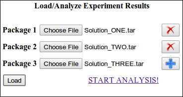
Figure 1. result analysis and performance comparison tool at glance.
Result Analysis Section
Using the result analysis section, we visualize and compare the bandwidth of Node3 as seen by Node2 for different experiment runs. Click the ADD Graph button as shown in figure 1 above. It is also possible to create as many graphs as needed. Each graph is customized by three subsections. The first is database selection. Here we select different experiment runs that we need to visualize. For this tutorial, three distinct solutions were conducted in search of the optimal bandwidth over the link Node3 to Node2. Figure 2 shows the database selection view of the ISR experiment.
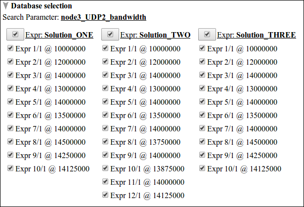
Figure 2. database selection view of the ISR experiment over three distinct solutions.
From the figure above, the search parameter node3_UDP2_bandwidth indicates the tune variable that was selected in the parameter optimization section of experiment execution tool. Moreover, The number of search parameters indicates the level of optimization carried, thus for ISR experiment it is a single parameter optimization problem. The other thing we see on the figure is solutions are grouped column wise and each experiment is listed according to experiment #, run # and specific search parameter value. For example Expr 10/1 @ 13875000 indicates experiment # 10, run # 1 and node3_UDP2_bandwidth=13875000 bit/sec. Before continuing to the other subsections, deselect all experiment databases and select only Expr 1/1 @ 10000000 from all solutions.
The second subsection, graph analysis, selects x-axis and y-axis data sets. To this end, the database meta data file is parsed into structured arrangement of groups, applications, measurement points, and metrics out of which the data sets are queried. Besides this, there are three optional selection check-boxes; AVG/STDEV, LABEL, and RANGE. AVG/STDEV is used to enable average and standard deviation plotting over selected experiments. LABEL and RANGE turns on and off plot labeling and x-axis y-axis range selection respectively.
The last subsection is custom graph analysis and it has similar function like the graph analysis subsection. Compared to the graph analysis subsection, SQL statements are used instead of parsed XML metadata to define x-axis and y-axis data sets. This gives experimenters the freedom to customize a wide of range of visualizations. Figure 3 shows graph analysis and custom graph analysis subsections of the ISR experiment. For graph analysis, begin_interval and size (i.e. bandwidth) from Node2 group, iperf_UDP application, transfer measurement point are used as x-axis and y-axis data sets respectively. For custom graph analysis, mean interval and size (i.e. bandwidth) are used as x-axis and y-axis data sets respectively.
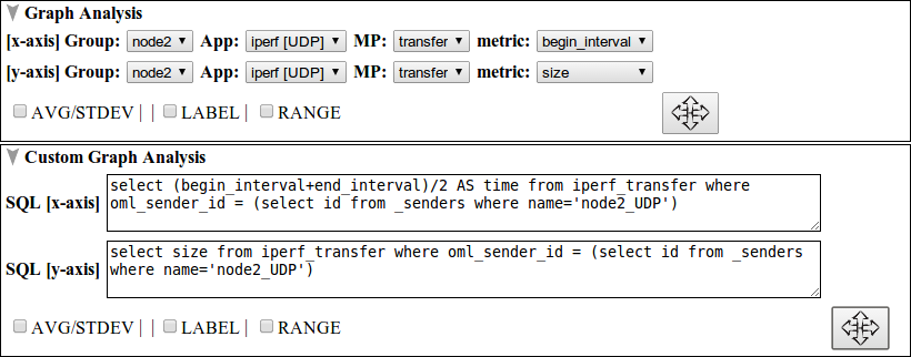
Figure 3. graph analysis and custom graph analysis subsection view.
Now click the arrow crossed button  in either of the graph analysis subsections to visualize datagram plot for the selected experiments. Figure 4 shows such a plot for six experiments.
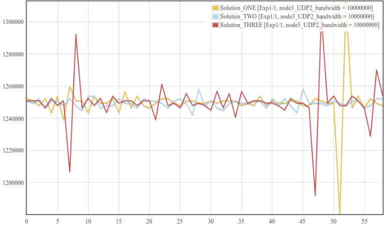
Figure 4. bandwidth vs. time plot for three identical experiments.
The first thing we see from the above figure is in each of the three experiments, Node2 reported almost identical bandwidth over the one minute time interval.Second the y-axis plot is zoomed within maximum and minimum result limits. Sometimes, however, it is interesting to see bandwidth plot over the complete y-axis range which is starting from zero up to the maximum. Click the RANGE check box and fill in 0 to 55 in the x-axis range and 0 to 1500000 in the y-axis range. Moreover, in repeated experiments one of the basic things is visualizing the average pattern of repeated experiments and see how much deviation each point has from average. Check the AVG/STDEV check-box (check the SHOW ONLY AVG/STDEV check-box if only AVG/STDEV plot is needed). Figure 5 shows the final modified plot when complete y-axis range and only AVG/STDEV plot is selected.
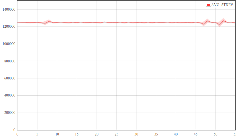
Figure 5. average bandwidth as a function of time plot from three identical experiments
Performance comparison Section
In performance comparison, a number of experiment metrics are combined and objective scores are calculated in order to compare how good or bad an experiment performs related to other experiments.
For this part of the tutorial, we create a simple score out of 100 indicating how much percent the receive bandwidth reaches and the transmit bandwidth. The higher the score the better the receive bandwidth approaches the transmit bandwidth and vise versa. Start by clicking the ADD Score button and a score calculation block is created ( Note: go further down to reach the score calculation section). A score calculation block has three subsections namely variable definition, score evaluation and database selection.
The variable definition subsection defines SQL driven variables that are used in the score evaluation process. For this tutorial, we create two variables one evaluating the average receive bandwidth and the second evaluating the transmit bandwidth. Click the plus icon twice and enter the following SQL command into the first text-area "SELECT avg(size) from iperf_transfer where oml_sender_id=(select id from _senders where name='node2_UDP')". For the second variable click the icon  to select variables from search parameters and select node3_UDP2_bandwidth.
The next subsection, score evaluation, is a simple mathematical evaluator with built in error handling functionality. Coming back to our tutorial, to simulate the percentage of receive bandwidth to transmit bandwidth, enter the string 100*(8*x1)/x2 in the score evaluation text-area ( Note: x1 is multiplied by 8 to change the unit from byte/sec to bit/sec).
Finally, database selection subsection serves the same purpose as was discussed in the result analysis section. Now press the arrow crossed button in the score evaluation subsection. Figure 6 shows the scores evaluated for the ISR experiment.
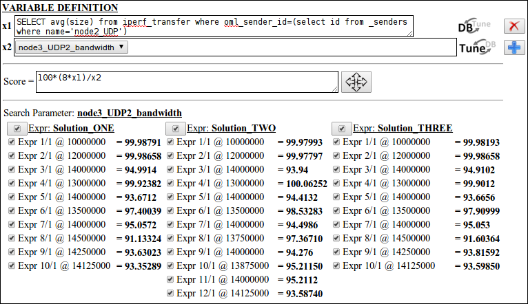
Figure 6. score evaluation section showing different configuration settings and score results for the ISR experiment.
Performance comparison is possible for identical search parameter settings among different solutions. For example comparing Expr1/1 @ 10000000 experiments from the three solutions reveals that all of them have receive bandwidth about 99.98% of the transmit bandwidth and thus they are repeatable experiments. On the other hand, the scores from any Solution show the progress of the optimization process. Recall the objective function definition (i.e. (8*x1)/x2 < 0.95 => stop when 8*x1 < 0.95*x2) in the ISR experiment such that the IVuC optimizer triggers the next experimentation cycle only when the receive bandwidth is less than 95% of the transmit bandwidth. Indeed on the figure above, search bandwidth decreases as the performance score decreases below 95%. Therefore performance scores can be used to show optimization progress and compare among different Solutions.
| Attachment | Size |
|---|---|
| Solution_ONE.tar | 380 KB |
| Solution_TWO.tar | 450 KB |
| Solution_THREE.tar | 380 KB |
Experimentation methodology
This document below describes the CREW methodology for experimental performance evaluation. While the scope of the CREW methodology is the analysis of cognitive networking and cognitive radio solutions, the methodology is broader in a sense that it may be applied to a wider range of (wireless) networking experiments.
The content in this document is largely taken from CREW deliverable D4.2, which is yet to be approved by the European Commission. As soon as deliverable D4.2 is approved, the latter document will supersede the information contained in this document.
| Description | Download |
|---|---|
| CREW methodology for experimentation |  |
In addition to the methodology described in the above document, (a growing list of) more concrete hints and best practices on using the different testbeds is found below.
Experiments using iMinds w-iLab.t
a.General comments
- Extensive documentation on the w-iLab.t testbed was added to the CREW portal. Prior to executing any experiment on w-iLab.t, read the documentation on http://www.crew-project.eu/portal/wilabdoc carefully and go through the various tutorials that are listed. Please also read the FAQ section at http://www.crew-project.eu/content/faq.
- As listed on the portal, there are two locations in the w-iLab.t testbed. Choosing the right location for your experiment is an important choice, as –at the moment of writing- the sensor side of the testbed is not yet 100% compatible, and the tools that are used to control the environments are not (yet) identical. As such, while far from impossible, porting experiments from one environment to another environment takes time.
b.Good practices for experiments involving USRP devices
- The USRP is one of the important cognitive components in the w-iLab.t testbed. Each USRP has a specific IP address. Unlike the standard configuration, the USRPs here are first attached to an high speed switch and then to interfaces of several quad-core servers. The alternation of this configuration should be avoided in any case, since it might influence the internal network address for other devices.
- As the quad-core servers for controlling USRPs are shared by multiple users, it is a good practice to save the operating system’s image each time after the design and experiment, next time reload it again.
- Timing is a crucial factor for cognitive experiments. OMF control and manage framework keeps very good log by default. The log file is located both on the central experiment controller and on the distributed nodes, which can provide precious information for debugging and improvement.
- Repeating experiments with nodes at different locations of the testbed is also a good practice. Since not all nodes in w-iLab.t have line-of-sight connection, even the relative positioning of antennas on different nodes can some time affect the experiment result.
- All the Wi-Fi interfaces in w-iLab.t Zwijnaarde have a 10 dB attenuator attached, which makes it easier to form multi-path scenario. Of course this fact should be kept in mind for experiments including power or pathloss measurement. Note that no attenuators are installed on the USRPs.
Experiments using the IMEC sensing engine
There are 2 instances of the IMEC sensing engine (both are present in the iMinds testbed), the differentiator between the two instances is the radio board. A first version uses the Wireless Open-Access Research Platform (WARP) radio board and the second version uses the IMEC SCALDIO IC. The main difference between the two instances is the RF range, the WARP radio board can only measure in the 2.4 and 5 GHz ISM, whereas the SCALDIO IC can measure signal between 0.1 and 6 GHz. Therefore it is mandatory that the experimenter selects the device that suits the experiment’s frequency requirements. Beware that in the iMinds testbed there are 10 IMEC sensing engines installed and only 2 SCALDIO sensing engines.
Before starting the actual experiment it is good practice to run a calibration/characterization phase if possible. In most cases the ideal sequence for this would be to execute a measurement of known signal and the absence of the signal, e.g. executing a spectrum measurement with a known signal connected directly to the input and executing a spectrum measurement with a 50Ω terminator connected to the antenna input. These measurements can afterwards serve as a reference measurement and can provide e.g. the noise floor of the spectrum sensing operation. Unfortunately connecting a known signal is directly to the input is only possible when one has full physical access to the device, which is not always the case when accessing a testbed remotely. In this case we would recommend transmitting a continuous signal with only one source at a time and measure this signal with all sensing devices. Afterwards the user can repeat this with sources at several locations in the testbed to check if all sensing devices can pick up the signal.
Experiments using IRIS and the CR testbed at TCD
- Everything in the testbed has an exact place
- Each USRP and node has been assigned a table and number.
- Unused daughterboards will be placed in proper storage places.
- Everything goes back to the exact place after any experiment that causes it to be moved.
- Clonezilla is used on all nodes meaning that nodes will be reset to a specific version of IRIS on startup.
- Bearing this in mind everyone should take care to store data in the data partition and not elsewhere on a node as it will be lost otherwise.
- The firmware in the USRPs will be updated when a new release becomes stable. All hardware will be updated at once rather than a subsection of hardware.
- If it is found that any piece of equipment gets broken, or if there is an issue with its functionality (e.g. only works for a certain bandwidth or really low powered) the IRIS testbed users mailing list iris-testbed-users@scss.tcd.ie must be informed. This will be relayed this to the wider group and a note will be made of this on the appropriate wiki pages https://ntrg020.cs.tcd.ie/irisv2/wiki/TestbedInventory.
- All experiments must be scheduled using the Google calendar <ctvr.testbed> specifying all of the following:
- Name of experimenter
- Date and time of booking
- Testbed node number(s)
- Daughtboard(s) of use
- Frequency range(s) of use
- The testbed should not be used for simulations.
- The testbed room should be kept secure.
- Testbed users should sign up to the following mailing lists:
- IRIS support mailing list https://lists.scss.tcd.ie/mailman/listinfo/iris2
- IRIS testbed users mailing list https://lists.scss.tcd.ie/mailman/listinfo/iris-testbed-users for enquiries regarding the Iris testbed.
- IRIS commit mailing list https://lists.scss.tcd.ie/mailman/listinfo/iris2commit for commit notifications.
- Short descriptions of all experimental work using the testbed should be provided in the projects section of the IRIS wiki https://ntrg020.cs.tcd.ie/irisv2/wiki/ActProjects.
Experiments using TWIST at TUB
The 2.4GHz ISM band is usually very crowded. Although, we have managed to switch the university wireless access network (eduroam) to the 5GHz ISM band and focus the TWIST testbed activities on 2.4GHz band, being now reserved only for experiments, it is a good practice to monitor the frequency band of interest for unsuspected interferences. The university network was moved to 5GHz band only in the building with the testbed and it is still possible to catch transmissions coming from either other buildings nearby or outdoor mesh network. It is possible to use low cost spectrum analyzers, WiSpy’s, in the TWIST testbed to perform constant monitoring of the spectrum, while performing an experiment. This enables validation of an experiment, before, during and after an experiment as explained in 3.3.1.
Proper description of the experiment and publishing the raw data adds to the transparency of the results. It makes it easy to verify if the experiment performed correctly as well as gives the possibility to explore other aspects using the same set of data. The proper description of the experiment should enable the repetition of the same it later on, also by another experimenter.
There is a set of good practices for experiments involving TUB testbed hardware:
- Extensive documentation on the TUB testbed can be found on the CREW portal. Prior to executing any experiment in the TUB testbed please read the documentation on http://www.crew-project.eu/portal/twistdoc carefully and go through the various tutorials that are listed. Please also read the FAQ section at http://www.crew-project.eu/content/faq.
- There are dedicated mailing lists, which users can subscribe and ask questions concerning TWIST. The following mailing lists are available:
- <twist-users AT twist.tu-berlin.de> for discussions on TWIST setup and usage
- <twist-devel AT twist.tu-berlin.de> for discussions on TWIST software development (more information can be found online: http://www.twist.tu-berlin.de/wiki/TWIST/Support/MailingLists)
- Before an experimenter is granted access to TWIST she/he must agree to the TWIST terms of usage, which includes
- the nature of the intended experiments (due to the privacy implications)
- commitment to a reciprocal access to eventual testbed resources; and
- agreement on proper acknowledgement of TWIST in the produced publications.
- All experimenters must be registered via the TWIST web interface
- When the experimenter uses TWIST she/he can reserve a time slot to have exclusive access to some hardware using a dedicated registration service (via the TWIST web interface)
- The integration of WiSpy spectrum devices has only recently been finished, therefore spectrum sensing is in an alpha-stage. Experimenters may be asked to provide TUB with feedback after using WiSpy monitoring during an experiment. This allows TUB to improve the service.
- During an experiment on TWIST experimenters can access data from their system under test in real-time over a separate channel; the connection is realized over SSH and the password will be provided on request.
- Repeating experiments with nodes using different topologies is a good practice. Furthermore, since the TUB building is a public building that is usually closed after working hours (and on weekends) it is a good practice to compare experimental results for working vs. non-working hours. This allows investigating effects due to external (uncontrolled) RF interference but also to mobility of the environment (affecting multipath fading, etc.).
Experiments using the LTE/LTE advanced testbed at TUD
a.Before the experiment:
- Contact the testbed staff, make sure the hardware is compatible (frequencies) and the testbed supports all features necessary for the intended experiment
- Make sure there will be enough testbed hardware available (indoor/outdoor?)
- If reasonable, ask for reference signal files to check compatibility with external hardware
- Get familiar using the spectrum analyzer R&S FSQ
- Prepare UE/eNB configuration files or ask testbed staff to do it
b.During the experiment:
- Carefully check the setup
- Use a terminator when there is no antenna/cable plugged
- Check if all cables are ok
- Make sure you are using the latest version of the config tool to configure the hardware
- Keep a record of the config files you use as you are changing parameters
- Check the signal on the spectrum analyzer, several things can be validated that way
- If in nothing else seems to work reboot and reconfigure the UE/eNB prototype hardware
- When in doubt, ask the testbed staff
c.After the experiment:
- Put everything back where you took it from
Experiments using LOG-a-TEC testbed (JSI)
- All experiments have to be scheduled and approved on LOG-a-TEC web portal: https://crn.log-a-tec.eu/. If unavailable or unresponsive, please notify the testbed staff.
- The communication between application and the testbed is based on a custom protocol, which is abstracted by a proxy server based on standard HTTP protocol.
- Users have the opportunity to interact with the testbed in three different ways, depending on the difficulty of performed task:
- by using pre-prepared GET and POST requests (trivial),
- by using a web GUI to write GET and POST requests one by one or to put more in a text file and upload it to the server (medium),
- by using a programming language with a HTTP client to write custom code based on GET and POST requests to the sensor network e.g. Python or Java.
- Several firmware options are preinstalled on VESNA platforms deployed in the LOG-a-TEC testbed and can selected for execution. If an experiment requires a new firmware, this should be prior to upload and execution in the LOG-a-TEC testbed at JSI testbed for proper functioning and compliancy with the hardware used. This testing is required to ensure that the reprogrammed devices are able to join the control network and accept commands from it.
- In case any of the nodes is inaccessible, please notify operators of the testbed.
- In LOG-a-TEC testbed there are 3 types of spectrum sensing modules installed, with only one available in the particular device. Make sure that the devices used are equipped with the modules required the experiment.
- When in doubt or experiencing unexpected behavior, please notify and investigate with the testbed staff.
- The radio environment on LOG-a-TEC testbed is not controlled, so unexpected interference can appear during experiments, especially in the crowded 2.4 GHz band. From the two clusters of the LOG-a-TEC testbed, one is located in the city center and the other in the industrial zone. Their interference profiles may be substantially different and can differ with respect to time of day (e.g. less Wi-Fi users in the night). In case of potential or experienced problems, please coordinate with the testbed staff.
- When planning an experiment keep in mind that the control network in LOG-a-TEC testbed is based on a ZigBee network, which occupies only one channel in the 868 MHz frequency band and offers only a low transmission rate. On average 1 kB/s transmission rate can be achieved, and the latency of the network is a few hundred milliseconds. If the data cannot be collected in real-time, SD card storage available in every device should be used.
- The storage on the SD card can hold traces up to 1 MB. This is enough for storing the results of at least 20 minutes of sniffing in the ISM bands, and 8 hours of sniffing in the UHF bands. During one experiment, more traces can be created, if necessary.
- Time synchronization of the nodes in the network is not implemented explicitly, so be aware of the possible drift between the traces. For achieving better synchronization, one can start all of the sniffing nodes planned to be used in an experiment, and then transmit a short synchronization burst which to be recorded by all sniffing nodes. Then by using the synchronization burst, the collected traces can be aligned.
- The GRASS-RaPlaT extension can be used either in experiment planning via simulations or cross validation of simulation and experiment results. Several dedicated processes are pre-prepared and available for the execution. Most common way of accessing the functionalities is through the LOG-a-TEC portal, which calls proper Linux processes and latter graphically visualizes the results. The GRASS-RaPlaT web interface can also be made accessible upon user request. In case experiencing problems, please contact testbed staff.
Experiments using the TCS sensing platform
a.Before going on the field
- Make sure to have all the necessary cables in order to connect the four parts of the test bed (Laptop, acquisition board, receiver, antennas)
- Make sure the hardware is compatible in frequencies with the LTE network to be sensed
b.Once on the field
- Make sure all cables are plugged correctly
- Switch on the acquisition board before booting the laptop.
- Switch on the receiver before launching the SMARTAIR3G software.
c.Acquisition part
- Run the setup test in order to verify that everything works correctly
- Set the acquisition parameters i.e.
- Acquisition length
- Number of antennas
- Path for file storage
- Generic file name
- Change the center frequency to the one to be analyzed
- Check on the time and spectral views that a signal is received
- Verify that the AGC works properly and that the signal is not saturating. If so, adjust the gain manually.
d.Analysis part
- Set the analysis parameters i.e.
- Number of antennas
- Precision of the analysis (number of frames used)
- Path for report file storage
e.After the experiment
- Switch of the laptop before unplugging any other equipment
Experiments using EADS Aircraft Cabin Mock-Up
The EADS aircraft cabin mock-up is a realistic replica of an Airbus A340 cabin using original equipment for the cabin interiors, such as seats, overhead compartments and lining material. The outside structure of the mock-up consists of wood. To make it useable for realistic wireless experimentation, all structural components have been coated with metal foil. In the technically relevant frequency range, due to the skin effect, the metallic foil has the same properties than solid metal parts would have regarding reflection and dispersion of electromagnetic fields. The interior of the mock-up as well as parts of the metallic coating are shown in Figure 23.
Although the mock-up is not part of the CREW federated testbed and not openly accessible, experiments referring to the special environment of an aircraft cabin can be performed according to explicit prior agreement.
Any kind of equipment can temporarily be installed in the mock-up, as long as it does not require irreversible modifications, causes damage at structure or interior, or interferes with the normal usage of the mock-up for tests and demos by EADS. 230 V power sockets are available at multiple sockets in the floor of the cabin and can be used to power the installed equipment. To reduce the occupation time of the mock-up, experimenters should have a precise concept for their planned tests and optimally should have performed a dry run before.
It is also possible to install components of the CREW federated testbed in the cabin mock-up for cognitive radio experimentation. This mobile testbed approach has been used for a series of internal experiments described in deliverable D6.2. Depending on the component selection, usage of all functionalities, such as the common data format or benchmarking is supported. Also a portal for remote access and remote experiment execution in principle can be set up (It is rather difficult to occupy the mock-up for longer time periods, so that in most cases a temporarily condensed experimentation campaign is preferred). It has been shown that installation of the mobile testbed can be done in a timescale of few hours to enable rapid experimentation in an aircraft cabin environment using the known CREW testbed components.
| Attachment | Size |
|---|---|
| methodology.pdf | 405.65 KB |
Wireless Testbeds Academy
The WirelessTestbedsAcademy GitHub account contains several repositories with simple code examples that can be run on one or more wireless facilities.
BasixTx/Rx: This repository describes several experiments that show the operation of a simple transmitter (Tx) and simple receiver (Rx) can be implemented using the APIs available on the individual testbeds.
BasicCR: This repository describes several experiments that show the operation of a simple cognitive radio example that can be implemented using the APIs available on the individual testbeds. For some testbeds, a docker image is available that contains all the necessary files and configurations to run the experiment.
BasicSensing: This repository describes several experiments that show how to do basic spectrum sensing using the APIs available on the individual testbeds. For some testbeds, a docker image is available that contains all the necessary files and configurations to run the experiment.
ChannelGain: This repository describes a simple channel gain experiment that shows how the gain between a transceiver and a receiver can be measured on a real testbed.
CrossTranscieverAPI: This repository contains the code for the WINNF transceiver facility implementation for SNE-ESHTER.
CDF toolbox: This repository contains the the CREW Common Data Format toolbox (Matlab) .
imec sensing engine in w-iLab.t Zwijnaarde testbed
Deployment
There are 7 imec sensing engine deployed in wilab2 in total:
5 imec sensing engines with WARP frontend are attached to the zotac nodes: 12,19,37,44,51 2 imec sensing engines with scaldio frontend are attached to the zotac nodes: 30, 41
This is shown in the figure below:
Each imec sensing engine has a unic spiderID and for scaldio frontend, it also has a frontend ID. The following table contains the configuration in w-iLab.t Zwijnaarde, to get more information see the SenisngEngineUserManual.pdf
| node | spider | frontend |
| 12 | 139 | 0 |
| 19 | 140 | 0 |
| 30 | 129 | 1 |
| 37 | 147 | 0 |
| 41 | 130 | 19 |
| 44 | 145 | 0 |
| 51 | 146 | 0 |
Use imec sensing engine within Emulab experiment
To use imec sensing engine, you need to have an emulab experiment swapped in with at least one of the nodes listed above. An example ns file with one wilab2 node is listed below:
The easiest way is to join the cognitiveradio project on emlab and after your experiment swap in, go to /proj/cognitiveradio/sensing/imecse folder
Content of the imecse folder under cognitiveradio project
1) setupscaldio.sh and setupwarpfe.sh are the scripts to program imec sensing engine
2) environment.csh contains the environment varialbes that need to be set
3) hardware, ztex contains the first level firmware required by the setupscaldio.sh or the setupwarpfe.sh
4) firmware and scaldio_files contains the firmware needed during run time by the sensing engine
5) includes, libaries contains the sensing engine header files and the compiled library for linux 2.6 64bit platform
6) apps contains an example application using the imec sensing engine
7) SensingEngineUserManual.pdf contains the detailed configuration of the sensing engine
8) oedl_example folder contains a simple example that uses OEDL script to control imec sensing engine
Configure imec sensing engine
To setup the sensing engine with WARP front end
1) source environment.csh
2) ./setupwarpfe.sh
To setup the sensing engine with scaldio frontend
1) source envrionment.csh
2) ./setupscaldio.sh
Example applications
The example apps in apps folder contains: Makefile main.c MAIN when run ./MAIN spiderid frontend, the application uses imec sensing engine to scan the 14 802.11g channels and print it out on stdard out
To create your own imec sensing engine application
1) source environment.csh
2) Copy apps, includes, libraries to your own home folder
3) adapt the main.c file
4) make
5) hopefully you have your own binary now