Experiment optimization is the heart of the CREW experiment execution tool. The efficiency of an experiment execution tool mostly depends on how it optimizes the different experiments to come and how fast it converges to the optimum. However, due a variety of problems in the real world, coming up with a single optimizer solution is almost impossible. The normal way of operation is to categorize similar problems into groups and apply unique optimizers to each one of them. To this end, the experiment execution tool defines a couple of optimizers which are fine tuned to the needs of most experimenters. Thus this paper explains the working principle of each optimizer supported in the experiment execution tool.

Step Size Reduction until Condition (SSRuC) optimizer

SSRuC is a single parameter optimizer aimed at problems which show local optimum or local minimum in the vicinity of the search parameter. Such kinds of problems are approximately described using two monotonically increasing and decreasing functions from either side of the optimum point. Figure 1 explains the problem graphically.

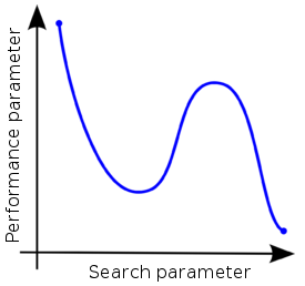
Figure 1. An example showing two local optimas with monotonic functions on either side of the optimum points

SSRuC tackles such problems using the incremental search algorithm approach [1]. Five parameters are passed to the optimizer. These are the starting, ending, step size of the search parameter, the step size reduction rate and the step size limit used as a stopping criteria by the optimizer. The optimizer starts by dividing the search parameter width into fixed intervals and performs unique experiment at each interval. For each experiment, measurement results are collected and performance parameters are computed. Next, a local maximum or local minimum is selected from performance parameters depending on the optimization context. If the optimization context is "maximization", we take the highest score value whereas for "minimization" context, we take the lowest score value. After that, a second experimentation cycle starts this time with a smaller search parameter width and step size. The experimentation cycle continues until the search parameter step size lowers below the limit. Figure 2 shows the different steps involved.

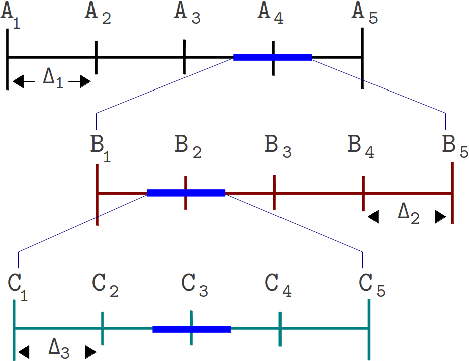
Figure 2. The different steps involved in an SSRuC optimizer over the search parameter width A₁ to A₅

Figure 2 shows the SSRuC optimizer in a three level experimentation cycle. In the first cycle, five unique experiments are conducted out of which the fourth experiment (experiment A₄ ) is selected. The second experimentation cycle works in the neighborhood of A₄ with a reduced step size ?₂ . This cycle again conducts 5 unique experiments out of which the second experiment (experiment B₂ ) is selected. The last experimentation cycle finally conducts 5 unique experiments from which the third experiment (experiment C₃) is selected and treated as the optimized value of the parameter.

Increase Value until Condition (IVuC)

IVuC optimizer is designed to solve problems which show either increasing or decreasing performance along the design parameter. A typical example is described in the experiment execution tool where video bandwidth parameter was optimized for a three node Wi-Fi experiment scenario. Datagram error rate was set as a performance parameter and the highest bandwidth was searched limited to 10% datagram error rate and below.

The algorithm used by IVuC optimizer is similar to the SSRuC optimizer in such a way that both rely on incremental searching. However, the main difference between the two is that the SSRuC optimizer performs a complete experimentation cycle before locating the local optimum value whereas the IVuC optimizer performs a local optimum performance check after the end of each experiment. Later on, both approaches refine their searching parameter range and restart the optimization process to further tune the search parameter. Figure 3 shows the different steps involved in IVuC optimizer.

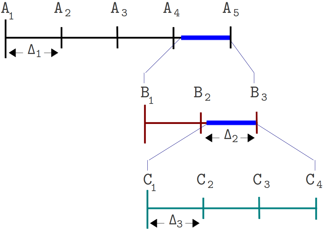
Figure 3. The different steps involved in an IVuC optimizer over the search parameter width A₁ to A₅

From figure 3, we see the three experimentation cycles each with five, three, and four unique experiments respectively. At the end of each experimentation cycle, performance parameter drops below threshold and that triggers the next experimentation cycle. At the end of the third experimentation cycle, a prospective step size ?₄ was checked and found below threshold, making C₄ the optimal solution.

SUrrogate MOdelling (SUMO)

Unlike SSRuC and IVuC, SUMO optimizer works on multiple design parameters and multiple design objectives. It is targeted to achieve accurate models of a computationally intensive problem using reduced datasets. SUMO manages the optimization process starting from a given dataset (i.e. initial samples + outputs) and generates a surrogate model. The surrogate model approximates the dataset over the continuous design space range. Next it predicts the next design space element from the constructed Surrogate model to further meet the optimization’s objective. Depending on the user’s configuration, the optimization process iterates until conditions are met.

The SUMO optimizer is made availabe as a MATLAB toolbox and works as a complete optimization tool. It bundles both the control and optimization functions together where the control function sitting at the highest level manages the optimization process with specific user inputs. Figure 4 shows SUMO toolbox in a nutshell highlighting the control and optimization functions together.

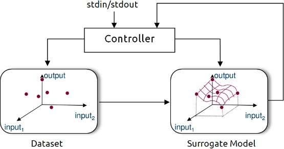
Figure 4.  Out of the box SUMO toolbox in a nutshell view

In the context of CREW benchmarking tools, the aim is to use SUMO toolbox as a standalone optimizer and put it inside the experimentation framework. This means starting from out of the box SUMO toolbox, the loop is broken, the control function is removed and clear input/output interfaces are created to interact with the controlling framework. Figure 5 shows how modified SUMO toolbox is integrated in the wireless testbed.

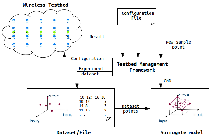
Figure 5. Integration of SUMO toolbox in a wireless testbed

The testbed management framework in the above figure controls the optimization procdess and starts by executing a configuration file. The controller pases configurations and control commands to the wireless nodes and measurement results are send back to the controller. After executing a number of experiments, the controller starts the SUMO toolbox supplying the experiment dataset which has been executed so far. The SUMO toolbox creates a surrogate model from the dataset and returns the next sample point to the controller. The controller again executes a new experiment with the newest sample point and generates a new dataset. Next the controller calls the SUMO toolbox again sending the dataset (i.e. one more added). The SUMO toolbox creates a more accurate surrogate model with the addition of one dataset. It sends back a new sample point to the controller and the optimization continues until a condition is met. It should be understood, however, that operation of the customized SUMO toolbox has not changed at all except addition of a number of blocks.

Having said about its operation, an example of wireless press conference optimization using customized SUMO toolbox is located on this link.

[1]. Jaan Kiusalaas, ”Numerical Methods in Engineering with MATLAB” Cambridge University Press, 01 Aug 2005, pp 144-146.